Lesson 2: Forecasting Methods in Project Management (Printer Friendly Format)
page 1 of 24
Lesson 2: Forecasting Methods in Project Management
Introduction
Forecasting is a critical and a fundamental process for any business, and project organizations are no exceptions. Forecasting is at the front end of the project environment. Forecasts of demand, activity times and the associated cost of these activities are prime inputs for planning the project and controlling project progress. Forecasting is the also one of the primary means for tracking project progress or for changing its direction if one is needed due to changes in the project environment. For example, forecasting technology will enable a project organization to rapidly respond to changes in the technological environment of the project is to ensure that changes in technology do not make the current project's facility obsolete. In this lesson, you will learn about the types of forecasts that are needed in a project environment and some of the important techniques that can be used to generate such forecasts.
Objectives
After completing this lesson you should be able to:
- Understand the reasons for forecasting in projects
- Know the various forecasting methods that can be used in projects
- Learn a method for forecasting the S-curve
- Understand the need for technological forecasting
- Know the various methods for technological forecasting
page 2 of 24
2.1 Reasons for Forecasting in Project Management
The ability to look into the future and make a forecast of what is going to occur is a vital aspect of project management. To be forewarned is to be forearmed and making reasoned forecasts of significant project events is a primary tactic for holding the project on course or altering the course if the forecasts show a change of direction would be appropriate.
Forecasting in project management can broadly be classified divided into three categories. These are:
- forecasting individual events,
- forecasting the outcome or progress of either a process or a large group of activities, and
- forecasting technology.
All of three categories are somewhat different in character, although some of the forecasting methods can be used in all of them.
Forecasting individual events can exist in a typical project situation where estimates are made of the completion dates of individual
activities within the plan as the project progresses. However forecasting the outcome of the project as a whole is a different
process as the past history of the project needs to be created (assuming relevant data from the past has been collected and retained)
which can serve as the basis for generating subsequent forecasts to track project progress. Forecasts of individual, stand alone
events that are not the result of a string of events are generally forecast by opinion based methods, whereas events that are the
result of a process may be forecast by one of a number of trend extrapolation techniques. In addition, technological forecasting
should be another vital, ongoing activity in the project management discipline as rapidly evolving technology can render the current
project facility obsolete.
Within this basic division, two further distinctions can be made:
- Forecasting, where there is some measurable history to use as a basis for the forecast
- Forecasting, where there little in the way of history
page 3 of 24
2.2 Forecasting Methods for Projects
Forecasting methods for projects fall into two broad categories:
- Qualitative
- Quantitative
Qualitative methods are used where no reliable, historical or statistical data are available. On the other hand, quantitative
methods are employed when measurable historical data is available. Let's begin by looking at qualitative methods.
page 4 of 24
2.2.1 Qualitative Forecasting Methods
The three primary approaches used in qualitative forecasting are the expert opinion approach, the Delphi method, and the market
survey approach.
The expert opinion approach is simple and easy to implement. For example, for many of the stand-alone, one-time activities that
take place in a project, an opinion based forecast is all that is either necessary or desirable. The opinion of the person who
is most knowledgeable in that field is sought. Furthermore, if a project is brand new, the likes of which have never been seen
before and for which no historical data is available, then the only recourse for a project manager is to seek the opinion of an
expert to get a forecast or an estimate regarding the concerned event or activity.
The disadvantage of relying on the opinion of a single expert is the inherent element of bias. Further, larger issues in the project
may arise where an opinion based forecast of a single expert may be not be adequate. This can occur with forecasts involving such
things as the timing of the introduction of a new technology into the market place or a change in public behavior as these could
have a significant bearing on the decision to start a project or the timing of market entry. When a new product is introduced it
can become a guessing game as to how the market will respond and how and when competitors might respond. Answers to questions such
as these may require the opinions of several experts, perhaps across a range of subjects, not simply an opinion from those closest
to the job. In such cases, the Delphi method may an appropriate forecasting method.
Devised by the Rand Corporation in the U.S., the Delphi technique is a popular method of qualitative
forecasting that generates a view of the future by using the knowledge of experts in particular fields. The name derives from the
ancient Greek Oracle of Delphi that was supposed to foretell the future. The steps of the Delphi method are as follows:
- Questionnaires are circulated to the team members, who may not be aware of each others' identities, and each is invited to
make his own prediction of future progress in a particular field. As far as possible, projections must be quantified and the
questions must be framed accordingly: e.g., what proportion of all households do you expect to have a personal computer by
the year 2010?
- After the first round of replies, the results are analyzed statistically (giving the distribution of responses) and the results
re-circulated; panel members are asked to reconsider their views in the light of the new statistics. If their view lies outside
the inter-quartile range, they must either revise their opinion or give their reasons for their extreme view; this will
be seen by the other panel members. This process can be repeated for a third or fourth round until a consensus of opinion is
obtained.
Results of Delphi studies are given in the form of timescales and probability levels for the feature being forecast. Some large
corporations have used the method for assessing long term trends and the development strategies that may be open. Research by the
Rand Corporation indicates that with current technologies and trends, the Delphi panel does tend to move towards a consensus view
which is generally correct, but there tends to be less accuracy when forecasting new developments. On occasions, no consensus view
is obtained after several rounds.
The market survey approach is the third qualitative approach that can be used to generate forecasts of project
events. This approach involves surveying past customers or potential customers about any plans they may be considering the future.
The project organization's marketing staff is perhaps the ideal source to obtain such information because of their direct contact
with customers. In addition, the marketing staff, along with the procurement staff, which is in direct contact with suppliers,
can also provide market intelligence reports regarding competitors who are contemplating new projects or new technologies.
page 5 of 24
2.2.2 Quantitative Forecasting Methods
Quantitative techniques of forecasting are appropriate in project situations where measurable, historical data is available and is usually used in forecasting for the short or intermediate time frames. These techniques can be classified into two broad categories:
- Time series analysis
- Causal methods
Let's take a look at each of these in turn.
page 6 of 24
Time Series Analysis
A time series is defined as a sequence of observations taken at regular intervals over a period of time. For
example, for a project organization such as Rolls-Royce, the monthly demand data for a particular type of aircraft engine over
the past ten years would constitute a time series. The main theme underlying time series analysis is that past behavior of data
can be used to predict its future behavior. However, in order to use time series analysis, we need to know about the three of the
important components that can constitute the time series of a project environment. These are trend, cycle, and the random components.
Trend is the long term movement of data over time. This definition implies that time is the independent variable and the data or set of observations we are interested in is the dependent variable. When we track data purely as function of time, there are several possible scenarios. First, data may exhibit no trend as shown in the example below. In this case data remains constant and is unaffected by time.
Time Period |
1 |
2 |
3 |
4 |
5 |
Data Value |
30 |
30 |
30 |
30 |
30 |
The second possible scenario is linear trend. In this case, data as a function of time has a linear relationship as shown in the example below. The table above shows that rate of increase data between successive time periods is a constant two units. This series is called an Arithmetic
Progression. It should be noted that data can also exhibit negative linear trend with a rate of decrease between successive observations.
Time Period |
1 |
2 |
3 |
4 |
5 |
Data Value |
30 |
32 |
34 |
36 |
38 |
The behavior of data over time may also exhibit a trend pattern that is nonlinear such as exponential growth or decay .
An example of observations that have an exponential growth pattern is shown in the table below. In this case, each successive data
value is twice its previous value. In this example each pair of successive observations have a common ratio. Such a series is called
a Geometric Progression.
Time Period |
1 |
2 |
3 |
4 |
5 |
Data Value |
30 |
60 |
120 |
240 |
480 |
In the case of exponential decay, each succeeding observation decreases by some constant factor. This is another form of the Geometric
Progression and a sort of pattern that is observed with such phenomena as the decay in radiation levels from nuclear activity.
The measure frequently used in exponential decay is the "half-life." It is the time it takes for the dependent variable
to decay to half its original value. An example of exponential decay is presented in the table below. In this example of exponential
decay, the half-life is one period.
Time Period |
1 |
2 |
3 |
4 |
5 |
Data Value |
400 |
200 |
100 |
50 |
25 |
Seasonal variations can be another component of a time series. These are periodic, short term, fairly regular fluctuations in data caused by man-made or weather factors. The increase in demand for candies during the Christmas season is an example of seasonal variations in data. Cyclical variations in a time series are wave-like oscillations in data about the trend line and typically have more than one-year duration. These variations are often caused by economic or political factors. Random variations are variations in data not accounted for by any of the previous components of the time series. These variations cannot be easily predicted and are only after the fact. In forecasting, these variations are accounted for as an error term. The decrease in demand for a company's product due to a plant shutdown caused by a labor strike is an example of a random variation in demand.
In addition to the qualitative and quantitative classification discussed above, forecasting methods can also be classified based on time frame. These are short term and intermediate term forecasting methods. Forecasting for the long term is typically done using by the qualitative methods discussed earlier in this lesson. We will now explore the various forecasting techniques that can be employed for the short and intermediate term forecasting.
page 7 of 24
Short Term Forecasting Methods
In many situations, a forecast is often required of what will happen in the immediate future without much regard for what will
happen in the longer term. This is a common situation with many production processes where a forecast has to be made at the end
of one period of the orders that are going to be received in the next so that production schedules can be set for the next period.
For the most part, short term forecasts do not require sophisticated analysis techniques. If historical data in the form of a time
series exists, then the forecaster can use any of the following techniques for short term forecasting: the naïve
approach, simple averages, moving averages, and exponential smoothing. Let's discuss each in detail.
page 8 of 24
Naïve Approach
In this approach, the forecast for the current period is the value of the previous observation of the time series. This approach
to forecasting has found wide use due to its simplicity. It can be used with a time series that may be stable, has seasonal variations
or has a trend component. In a project situation, this approach, in the absence of any other information, could be used for predicting
the number of staff available to perform activities in the next reporting period. Also, in the case of a resource scheduling routine
in use with a reporting period as short as one week, the naive forecast may be the most appropriate forecasting method for planning
next week's work and allocating staff to tasks. Using this approach, the forecast for
period t+1 is,
Ft+1 = At, Where
F t+1, is the forecast value for period t+1, and At,
is the actual value at time t.
page 9 of 24
Simple Averages
In simple averages, the next period's forecast is the average of all previous actual values.
In this case, the underlying assumption is that all history has a bearing on the most recent events. The fluctuations that are
seen from period to period are assumed to be merely random events that cannot be predicted with any certainty. In practice, this
method will damp out all fluctuations and as the data series becomes increasingly long, it will become increasingly less sensitive
to any recent movements in data. It would be most appropriate to use this approach where there are considerable random variations
in the observed values but no long term evidence of either a rising or falling trend. The averaging techniques in such cases smooth
out the time series as the individual high and lows cancel out each other. Consequently, the forecast value over time will become
increasingly stable. The biggest disadvantage, however, is that if trend is present in the time series data, the averaging technique
will lag the forecast. In other words, in the presence of an increasing trend, the use of the simple averaging technique will understate
the actual value; and in the presence of a negative trend, it will overstate the actual value. Projects, however, mostly encounter
situations that are not usually stable and hence this method might not be an appropriate forecasting technique for a typical project
situation.
page 10 of 24
Moving Averages
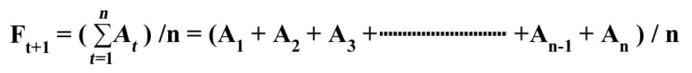
In this method the next period's forecast is the average of the previous n actual values.
Ft+1 =  actual
data values for n previous periods / n)
actual
data values for n previous periods / n)
i.e., Ft+1 = (At + At-1 +
At-2 + -------------- +A t-(n-1) ) / n
With this method the assumption is that the most recent events are the best indicators of the future with significant random fluctuations in the time series. This approach produces a moving average that is relatively more sensitive to recent movements in data and forecast responsiveness can be increased by reducing the value n. As this method uses only the most recent periods that are relevant, it greatly reduces the problem of forecast lag inherent in the simple averaging technique. The choice of the number of data values to be included in the moving average is arbitrary and is left to the judgment of the forecaster.
It should be noted, however, that while the moving average method uses the data from most recent periods, it still assigns equal
importance to all periods of data included in the base of the moving average. Consequently, even with this method there is bound
to be some forecast lag. This problem can be resolved to a certain extent by using an extension of the moving average called the weighted
moving average. In this method, the forecaster assigns more weight to most recent values in the time series. For example,
the most immediate observation might be assigned a value of 0.5, the next most recent value a weight of 0.3, and so on. The sum
of the weights, however, should be equal to 1. For example, the forecast using a weighted moving average with four recent periods
(n = 4) using weights of w1 = 0.5, w2 = 0.3, w3 =
0.2, w4 = 0.1, is given by:
Ft+1 = F5 = w1A4 + w2A3 + w3A2 + w4A1 = 0.5A4 + 0.3A3 + 0.2A2 + 0.1A1
page 11 of 24
Exponential Smoothing
In this method the next period's forecast is a weighted average of all previous observations that gives progressively less weight to older observations. Forecasts using exponential smoothing are simple to compute; thus, it is a very popular forecasting method that can be made as sensitive as required. This approach is called exponential smoothing because the forecast that is generated is made up of an exponentially weighted average of all previous observations. The averaging techniques discussed earlier are known as "smoothing" processes as they attempt to remove the random fluctuations from the time series so that the underlying trend can be seen more clearly and can thus be used for making a forecast that is not subject to random swings. Exponential smoothing was invented by R. G. Brown in the 1950s to make short term forecasts, primarily for the time period following the latest observation. The exponential smoothing formula is given by:
 , where
  is a smoothing factor, a fraction between 0 and 1.
The weights attached to each observed value in the series of values that make up any
"forecast", Ft+1 form an exponential series with the greatest weight being attached to the most recent observation. The weight for each of the preceding observation decreases exponentially by a fixed fraction (1-).
The sensitivity of the forecast to changes in the most recently observed data is controlled by the factor . If is set to 1 the new forecast (smoothed value) will be equal to the latest observation and there will be no smoothing. The implication in this case is that the new forecast should respond immediately to changes in the actual observation seen in the most recent period. On the other hand, if is set to 0, then all variations in the actual value from the initial forecast is ignored and the new forecast remains the same as the previous forecast value. This implies that the actual value in the most recent period is purely a random occurrence and hence should be ignored. In practice, however, the value chosen for is between 0.1 and 0.3.
In order to initialize exponential smoothing, a forecaster needs two pieces of information--an initial forecast and a value for . The value of is left to the judgment of the forecaster. An initial forecast can be obtained using the naïve approach by assuming that it is equal to the actual value from the previous period. We will now go through a simple example of generating forecasts using exponential smoothing.
page 12 of 24
Example of Exponential Smoothing
Consider the time series with nine periods of data:
34, 38, 46, 41, 43, 48, 51, 50, 56
Use exponential smoothing to forecast the value for period 10.
Assume F2 = A1 = 34 and = 0.2.
Solution:
Using the exponential smoothing formula
New forecast = old forecast + (latest observation - old forecast),
the forecast for period 3 is given by:
F3 = F2 + (A2 - F2 ) = 34 + 0.2(38 - 34) = 34.8
Similarly, the forecast for period 4 will be:
F4 = F3 + ( A3 - F3 ) = 34.8 + 0.2(46 - 34.8) = 37.04
This process can be repeated for the remaining periods to get a smoothed series given below.
34, 34.8, 37.04, 37.83, 38.87, 40.69, 42.75, 44.20, 46.56
Thus, the forecast for period 10 is given by F10 = 46.56
It can be seen that this series does produce a smooth trend but it also shows a marked "lag." Sensitivity of the forecasts for the above example can be improved by changing the value of a to 0.5. In this case the smoothed series becomes:
34, 36, 41, 42, 45, 48, 49, 49.5, 52.75 and the forecast for period 10 is now given by:
F10 = 52.75.
The results obtained for these different smoothing factors are shown graphically in Figure 2.1 below. See the highly damped smoothing and the considerable lag associated with the forecasts generated using  = 0.2 when compared to = 0.5.
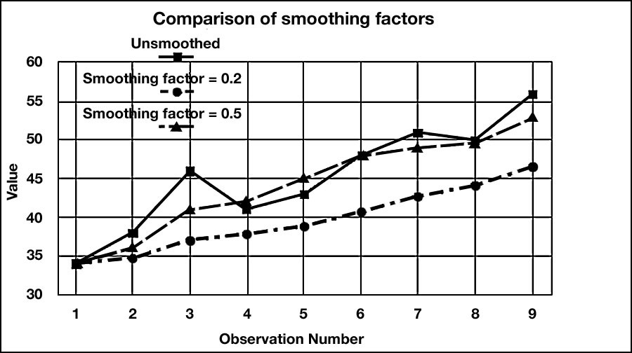
Figure 2.1 Comparison of Forecasts Generated by Different Smoothing Factors
page 13 of 24
Trend-Adjusted Exponential Smoothing
The exponential smoothing approach discussed above is an appropriate forecasting technique, if the time series exhibits a horizontal pattern (i.e. No trend) with random fluctuations. However, if the time-series exhibits trend, forecasts based on simple exponential smoothing will lag the trend. In such cases, a variation of simple exponential smoothing called the trend-adjusted Exponential smoothing can be used as a forecasting technique. "The trend-adjusted forecast (TAF) has two components:
- A smoothed error
- A trend factor
TAFt = St-1 + Tt-1 , where
St-1 = Previous period smoothed forecast
Tt-1 = Previous period trend estimate
TAFt = Current period's trend-adjusted forecast
St = TAFt +  (At - TAFt)
Tt = Tt-1 +  (TAFt - TAFt-1 - Tt-1), where and are smoothing constants
In order to use this method, one must select values of and  (usually through trial and error) and make a starting forecast and an estimate of the trend" (Stevenson, 2005).
page 14 of 24
Example of Trend-Adjusted Exponential Smoothing
For the data given below, generate a forecast for period 11 through 13 using trend-adjusted exponential smoothing. Use = 0.4 and = 0.3
Period |
1 |
2 |
3 |
4 |
5 |
6 |
7 |
8 |
9 |
10 |
Data values |
500 |
524 |
520 |
528 |
540 |
542 |
558 |
550 |
570 |
575 |
Solution: To use trend adjusted exponential smoothing, we first need an initial estimate of the trend. This initial estimate can be obtained by calculating the net change from the three changes in the data that occurred through the first four periods.
- Initial Trend Estimate = (528 - 500)/3 = 28/3 = 9.33
Using this initial trend estimate and the actual data value for period 4, we compute an initial forecast for period 5.
- Initial Forecast for period 5 = 528 + 9.33 = 537.33.
The forecasts and the associated calculations are shown in the table below.
Table 2.1 Forecast Calculations for the Trend-Adjusted Exponential Smoothing Example
Period |
Actual |
St-1 + Tt-1 = TAFt |
TAFt + 0.3(At -TAFt ) = St |
Tt-1 + 0.2(TAFt -TAFt-1 - Tt-1 ) = Tt |
5 |
540 |
528 + 9.33 = 537.33 |
537.33 + 0.3(540 - 537.33) = 538.13 |
9.33 |
6 |
542 |
538.13 + 9.33 = 547.46 |
547.46 + 0.3(542 - 547.46) = 545.82 |
9.33 + 0.2(547.46 - 537.33 - 9.33) = 9.49 |
7 |
558 |
545.82 + 9.49 = 555.31 |
555.31 + 0.3(558 - 555.31) = 556.12 |
9.49 + 0.2(555.31 - 547.46 - 9.49) = 9.16 |
8 |
550 |
556.12 + 9.16 = 565.28 |
565.28 + 0.3(550 - 565.28) = 560.70 |
9.16 + 0.2(565.28 - 555.31 - 9.16) = 9.32 |
9 |
570 |
560.70 + 9.32 = 570.02 |
570.02 + 0.3(570 - 570.02) = 570.01 |
9.32 + 0.2(570.02 - 565.28 - 9.32) = 8.41 |
10 |
575 |
570.01 + 8.41 = 578.42 |
578.42 + 0.3(575 - 578.42) = 577.40 |
8.41 + 0.2(578.42 - 570.02 - 8.41) = 8.41 |
11 |
|
577.40 + 8.41 = 585.81 |
|
|
The forecast for period 11 is 585.81.
page 15 of 24
2.3 Intermediate Term Forecasting
2.3.1 Linear Regression Analysis
One of the most useful techniques to evaluate and forecast the trend component of a time series is regression analysis. The trend component may or may not be linear. For example, the typical S-curves that we use in managing projects exhibit a non-linear trend. However, there are several project situations where the relationship of a project variable as a function of time can be assumed to have a linear trend. For example, forecasting the cost of an activity as function of time can be assumed to have a linear trend. While the assumption of linearity may not hold good in many situations over the long term, a linear relationship is often a reasonable assumption in the intermediate time frame. In such cases, linear regression analysis is a viable forecasting technique. It is also a useful methodology for determining the empirical relationship between two project variables if the underlying reasons if the relationship between those variables can be hypothesized to be approximately linear. In order to evaluate the trend component of a time series, we use linear regression analysis to develop a linear trend equation. This is the equation of a Straight Line is given by
Where b is the slope (gradient) of the line and a is the intercept with the y axis at t = 0, y t is the value of the project variable (for which we desire a forecast) at time period t and e is the forecast error.
The technique of linear regression analysis involves determining the values for "a" and "b" for a given data set. From a graphical perspective, the technique involves drawing a straight line that best fits the scatter of observed values that have been plotted over time (see Figure 2.1 below). "Best fit" means the difference between the actual Y-values and predicted Y-values are a minimum. However, positive differences will offset negative differences, hence we square the differences. Mathematically, the best fitting line is the one in which the sum of the squares of the deviations of all the data points from the calculated line is a minimum. In essence we are choosing a line where the scatter of the observed data about the line is at its smallest. The technique of "Least Squares Regression" minimizes this sum of the squared differences or errors. By using this technique, It can be shown (proof not given) that we can get formulas for a , the intercept and b , the slope of the regression line. These formulas are given below.
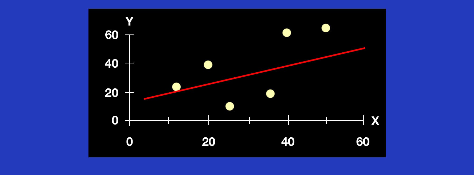
Figure 2.2 Line of best fit in regression analysis.
For a time series of n points of data where,
t = time i.e. the number of time periods from the starting point
y = the observed value in a given time period
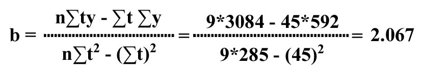
The slope b of the line is given by:
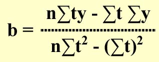 , and
, and
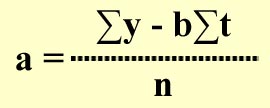
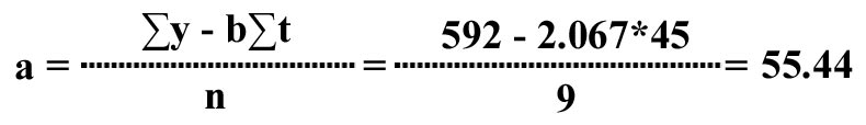
The intercept a is given by:
Interpretation of coefficients
Slope b is that the estimated Y changes by b, for each one unit increase in t.
Y-intercept (a) is the average value of Y when t = 0.
We will now look at a simple example for developing a linear trend equation using linear regression analysis for forecasting the trend component of a time series.
page 16 of 24
Example of Linear Regression
The historical data on the cost (in hundreds of $) for a project activity is given below. Develop a trend equation using Linear Regression Analysis and forecast the cost of this activity for period 10 and 15.
t |
y |
1 |
58 |
2 |
57 |
3 |
61 |
4 |
64 |
5 |
67 |
6 |
71 |
7 |
71 |
8 |
72 |
9 |
71 |
The calculations for determining the slope and intercept of the regression line are shown below
t |
y |
t*y |
t2 |
y2 |
1 |
58 |
58 |
1 |
3364 |
2 |
57 |
114 |
4 |
3249 |
3 |
61 |
183 |
9 |
3721 |
4 |
64 |
256 |
16 |
4096 |
5 |
67 |
335 |
25 |
4489 |
6 |
71 |
426 |
36 |
5041 |
7 |
71 |
497 |
49 |
5041 |
8 |
72 |
576 |
64 |
5184 |
9 |
71 |
639 |
81 |
5041 |
 t t = 45 |
y = 592 |
t* y = 3084 |
t2 = 285 |
y2 = 39226 |
The slope b of the line is given by:
The intercept a of the line is given by:
Hence the linear trend equation is given by:
yt = a + bt = 55.44 + 2.067t, and
The forecast for period 10 is given by
y10 = 55.44 + 2.067*10 = 55.44 + 20.67 = 76.11
For t = 15, y15 = 55.44 + 2.0667 *15 = 86.445
In the discussion and example above on linear regression analysis, the independent variable was t--the time period. However, the linear regression technique can also be used determine association or causation between two variables. In such cases, we use the notation x for the independent variable and y for the dependent variable. The linear regression equation in such cases would be of the form
yc= a + bxi, where
The slope b of the regression line is given by:
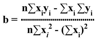 .
.
The intercept a of the regression line is given by:
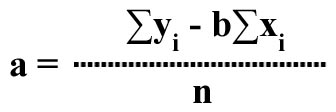 .
.
page 17 of 24
Evaluating the "Fit" of the Regression Line
The nest step in regression analysis after obtaining the regression line is to evaluate how well the model describes the relationship between variables, or how good is the line of "best fit". Three measures can be used to evaluate how well the computed regression line fits the data. These are: The Coefficient of Determination (R2 ), The Correlation Coefficient (r), and The Standard Error of the Estimate (syx)
The Coefficient of Determination (R2)
Three Measures of variation can be computed in linear regression analysis. These are:
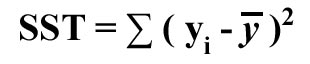
- Total sum of squares (SST)
This
measures the variation of the actual Y-values around the mean Y.
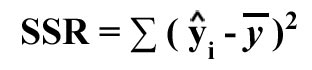
- Explained variation (SSR) or the regression sum of squares
This
measures the variation due to the relationship between X and Y, i.e., the difference between the mean Y and the predicted value Y using regression.
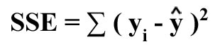
- Unexplained variation (SSE) or error sum of squares
This
measures variation not explained by regression, i.e., variation due to other factors or variables not included in the regression model.
- Coefficient of Determination (R2)
This
is the proportion of variation explained by regression (i.e., by the relationship between X and Y). The formula to compute R2 is:
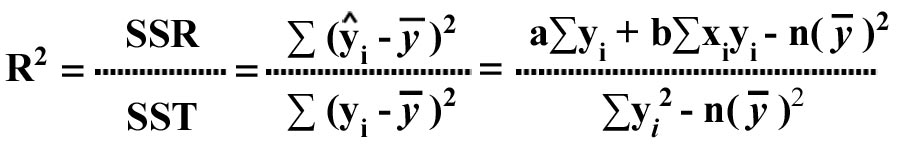
R2 takes on a value between 0 and 1. The higher the value of R2 the better is the line of fit.
page 18 of 24
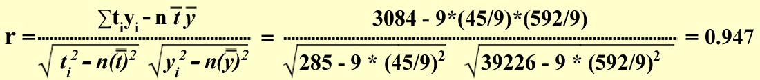
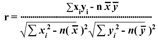
2.3.2 The Correlation Coefficient (r)
This statistic measures the strength of the relationship or association between x and y and takes on a value between -1 and +1. The closer the value of r to +1 or -1, the stronger the relationship is between the variables. The formula for r is given by:
page 19 of 24
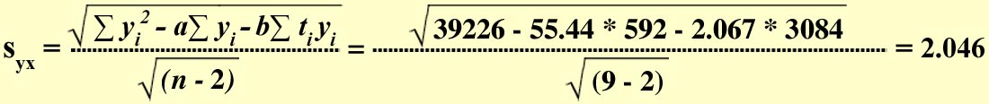
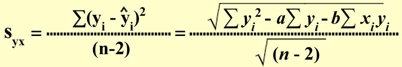
2.3.3. The Standard Error of the Estimate (syx)
Random variation which is the variation of the actual (observed) y values from the predicted y values (yi) is measured by the standard error of the estimate. The smaller the value of syx , the smaller the variation of the actual (observed) y values from the predicted y values (yi ), and hence better is the line of fit.
We will now compute the values for R2, r, and syx for the example problem on linear regression that we had solved earlier. As the independent variable in this example is t instead of x, we solve the above formulas for R2, r, and syx by substituting t for x. We have the following data from the example above.
All of the statistics indicate that the regression line obtained for example 1 is a very good line of fit.
page 20 of 24
2.3.4 Limitations in Forecasting Using Linear Regression
For the above example, If we plot the actual y values and the forecasted values using linear regression the graph is as shown below in Figure 2.3.
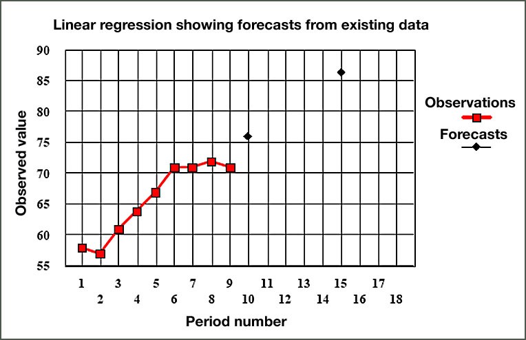
Figure 2.3 Forecasts using Linear Regression
In the above figure, notice that the forecasts using the regression equation shows a continuously rising trend. However, the pattern of actual observations, particularly over the last 4 periods, indicates a leveling off or perhaps even a down-turn. In such cases, the actual observations should, if possible, be investigated for any causes that can be discovered to account for this pattern. If there are substantial reasons for the behavior of the latest observations, these should always be taken into account when assessing the degree of credence to be placed in the regression forecast. It will also be clear from this example that the number of observations used to calculate the regression line can have a marked influence on the forecast. Where the number of observations is small, e.g., 4 or 5 values, serious errors can occur if the data happens to be behave badly.
In the example shown above, only one independent variable was considered. However, there may be occasions where several independent variables simultaneously influence the dependent variable. In such cases, an extension of linear regression technique called Multiple Linear Regression can be used. Multiple linear regression equation is of the form:
y = b0 + b1x1 + b2x2 + b3x3 + .... + bixi + e, where
x1, x2, x3 and xi, etc., are independent variables, and e is the error term.
b0, b1, b2, b3, and bi, etc. are termed the regression coefficients and they represent the amount by which y changes for one increment of xi assuming all other independent variables (x) are held constant. Students interested in learning more about this procedure should consult a statistics text. Two such texts are referenced on the final page of this lesson.
page 21 of 24
2.3.4 Limitations in Forecasting Using Linear Regression (continued)
There are, of course, many occasions when a simple linear model will not adequately describe the relationship between one variable and another. Unlike the linear case, there is no simple or direct method of defining the equation, although some computerized statistics packages will generate best fit curves according to a quadratic ( y=kx2 + c
) or a cubic ( y = kx3 + c ) law. Over short ranges of data where there is very little scatter, it is sometimes possible to get quite precise fits by a trial and error method, using different coefficients and taking successively higher powers of x to obtain an nth order regression. However, it must be remembered that such an empirical relationship only holds good within the range of actual data and cannot be extrapolated far beyond it.
Some curvilinear relationships can be described by the general expression:
Y - c = kxn
This expression generates a series of smooth curves with no turning points that can have a rising slope, when n is positive, or a downward slope when n is negative for x > 0. In the above expression, if we let y - c = y' , then we can transform the curvilinear equation into a straight line by taking logarithms of both sides of the above expression. Thus y' = kxn can be transformed into:
Logey' = Logek + nLogex
This relationship is most easily visualized using Log-Log graphical scales where it will be seen that a curved primary relationship can be transformed into a linear one. This is a useful method of generating an equation that will fit a series of data points and it also allows some well known curvilinear functions to be handled with greater ease. A particularly important example of the latter in engineering project work is the Learning Curve. For example, consider the two equations: y = 10x0.5 and y = 200x-0.33 . Plotted on linear scales, they appear as below.
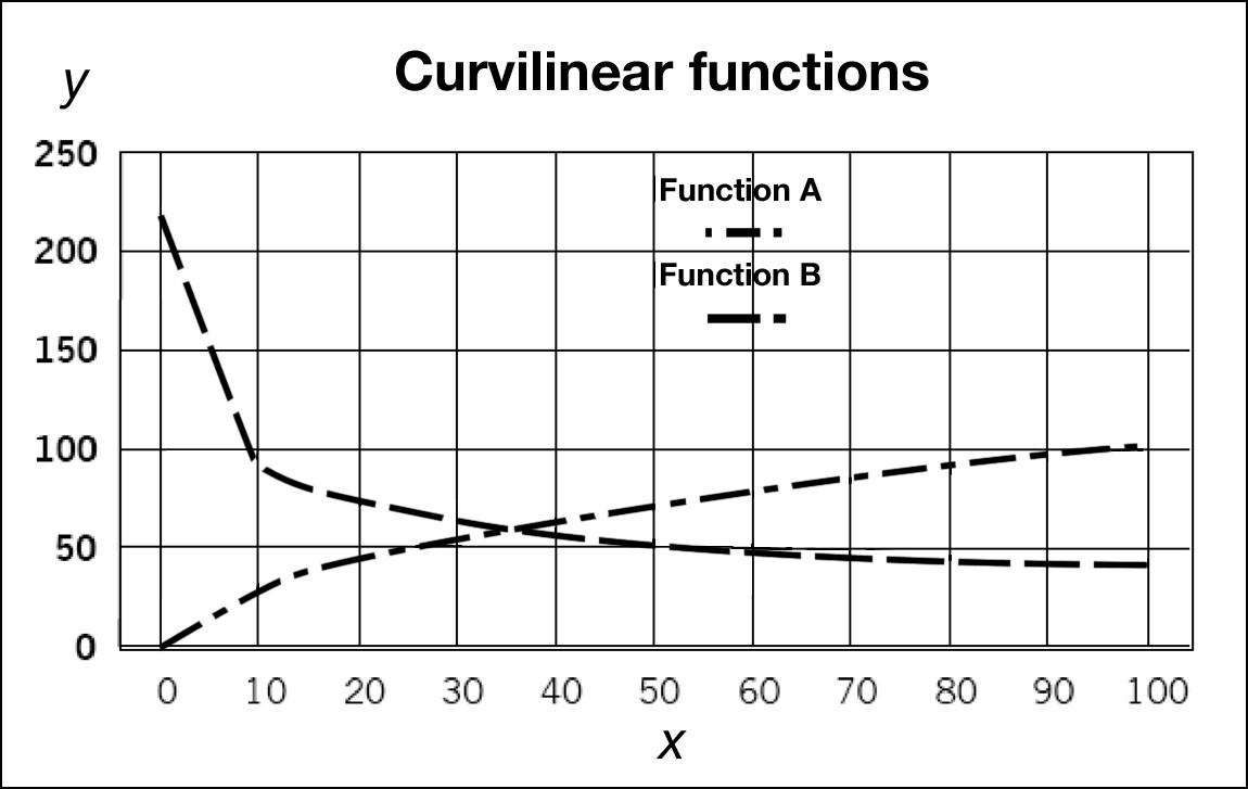
Figure 2.4 Plots of Functions (A) y = 10 x0.5 and (B) y = 200 x-0.33 on Linear Scales
Plotted on logarithmic scales, these curves now become straight lines as shown below in Figure 2.5.
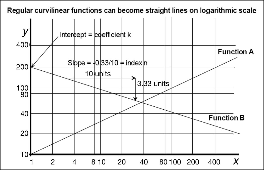
Figure 2.5 Plots of functions (A) y = 10x0.5 and (B) y = 200 x-0.33
Logarithmic plots are an extremely useful way of analyzing trends as many phenomena progress as a simple law of the form y = kxn. The rate of progress of the performance of some technologies can be clearly illustrated by linear logarithmic trends over time. Some frequency distributions can be illustrated using logarithmic plots. Once a straight line has been established, it is a simple process to compute the underlying equation. Furthermore, a straight line can be used as the basis for forecasting future values of the observed variable simply by projecting it forward. However, we must be careful about just how far ahead we can project to generate forecasts.
page 22 of 24
2.4 Forecasting the Project End Conditions
One particular issue that is always of concern to the project manager is the point at which the project will end. This can be of
supreme importance if the project has to be completed by some opening date that has been fixed well in advance, like the Olympic
Games, for example. One possible approach is the use of a Slip Diagram, which is a simple graphical technique based
on linear trend estimation. This method was covered in Module 1/MANGT 510 and hence the coverage here will be brief. The slip diagram
as a method of predicting the project end date is based on two sets of time series; a regular series of estimates of when the project
will end and a record of when those estimates are made. Plotting one data series against the other will reveal whatever pattern that
exists and if the relationship is linear, it can be extrapolated to produce a forecast of the completion date. Slip Diagrams can also
be used to forecast significant milestones in a project. A sample slip diagram is presented below in Figure 2.6.
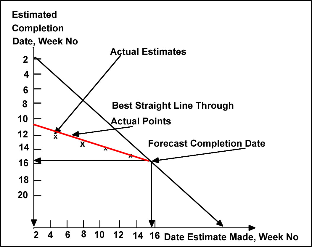
Figure 2.6 Construction of a "Slip Diagram"
page 23 of 24
2.5 S-curve Forecasting
The typical form of the relationship between project duration and expenditures incurred is S-shaped , where budget expenditures are initially low and increase rapidly during the major project execution stage before starting to level off again as the project gets nearer to its completion. The S-curve figure represents the project budget baseline against which actual budget expenditures will be evaluated. They help project managers understand the correlation between project duration and budget expenditures and a good sense of where the highest levels of budget spending are likely to occur. Forecasting the S-curve can help project managers generate estimates of expenditures during the various stages of the project duration.
The S-curve (also called a Pearl Curve) is based on what is known as the logistic or auto catalytic growth function . The Web site below has a complete discussion on the theory and the steps involved in S-curve forecasting. You are strongly urged to go over this document and follow through on the worked-out example. You may use this file to work on assignments for this lesson. See your online course Syllabus or Road Map for details.
http://leeds-faculty.colorado.edu/Lawrence/Tools?SCurve/scurve.xls
page 24 of 24
2.6 Technological Forecasting*
Technological Forecasting is defined as a process of predicting future characteristics and timing of technology. As the rate of change of technological capabilities are uncertain, It is imperative that project mangers use some methods to forecast future technology so that the project product that is developed using current technologies is not rendered obsolete. Two types of methods can be used for forecasting technology: Numeric-based Technological Forecasting Techniques and Judgment-based Technological Forecasting Techniques.
Numeric-Based Technological Forecasting Techniques
Numeric-based technological forecasting techniques include:
- Trend extrapolation that projects trend of data into the future
- Growth curves include invention, introduction and innovation, diffusion and growth, and maturity
- Envelope curves are a combination of trend extrapolation and growth curves
- Substitution model considers competing technologies developing over time
Judgment-Based Technological Forecasting Techniques
Judgment-based Technological Forecasting Techniques include:
- Monitoring is to track innovation to stay abreast of developing technologies
- Network analysis
- Explores applications of current research
- Determines how much research is needed to arrive at desired capability.
- Scenarios
- Forecast technology along with environment
- Can be used to forecast results of adopting a technological change
- Morphological analysis
- Systematically search for improvements in technology
- Plot technology vs. alternatives to achieve the technology
- Relevance trees look at a goal through a hierarchy of alternative tasks
- Delphi method
- Individuals in a group make anonymous estimates of when technology will be available
- Results fed back to the group and the process goes through a few iterations
- Cross-impact analysis is like the Delphi method, but model is stochastic
The particular model to be used should be appropriate for the environment of the firm and at a suitable cost.
You have now reached the end of Lesson 2. You should have a better understanding of forecasting and the forecasting methods available to you as a project manager. You should also have completed your reading assignment as specified on your syllabus. At this time,
return to your syllabus and complete any activities for this lesson. The next lesson will focus on cost estimation in project, including methods to ensure cost control.
Please Note: Section 2.6 was adapted from Meredith, J. R., and Mantel, S. J. (1989). Project Management: A Managerial Approach. 2nd Edition. New York: John Wiley and Sons.
References
- For Advanced Readers in Statistics:
Draper, N. R., and Smith, H. (1998). Applied Regression Analysis. 3rd Edition. New York: John Wiley and Sons.
- For Beginners in Statistics:
Levine, D. M., Stephan, D., Krehbiel, T. C., and Berenson, M. L. (2005). Statistics for Managers using Microsoft Excel. 4th Edition. Upper Saddle River, NJ: Prentice-Hall.
- Meredith, J. R., and Mantel, S. J. (1989). Project Management: A Managerial Approach. 2nd Edition. New York: John Wiley and Sons.
- Stevenson, W. J. (2005). Operations Management. 8th Edition. New York: McGraw-Hill/Irwin, p. 80.