
MBADM813:
Lesson 2: Distributions
Lesson 2 Overview
In the previous session, we looked at summary measures of data. Along with the measures of centrality (mean and median), we learned another important concept: variation (measured most often by standard deviation). Variation is inherent in nature; it is so ubiquitous that we often do not even realize it. For example, take your daily commute. Does it take the same amount of time even if traffic and weather conditions did not change? Of course not. If your average commute time is 30 minutes, it probably took you 28 minutes this Monday, 32 minutes on Tuesday, and may be 27 minutes on Wednesday. And on those rare occasions when an irresponsible driver texting while driving causes an accident and massive traffic jam, it may take you up to an hour.
The topic of variation brings us to our next discussion: uncertainty. Businesspeople must deal with this inherent variation all the time. Think about the auto parts supply chain. Suppliers promise to deliver within a time window, but the exact time of delivery may vary based on factors outside the control of even the most reliable supplier. So, the supply chain managers assess the risk of stockouts and maintain a minimum level of inventory all the time (known as safety stock). Higher/lower levels of risk would mean maintaining higher safety stock levels. If your inventory-carrying costs are high, you would want to be as precise as possible in your assessment of the likelihood of stockout.
Take another example: staffing decisions at an urban hospital emergency room. Admissions surge on late Friday and Saturday nights. The emergency room currently has three acute care rooms. The emergency room manager would like to know the chance that more than three patients will be admitted in an hour. Long wait times at the emergency room mean that patients suffer. This reflects badly on the hospital, affecting its reputation. If the chance is high, the hospital should invest in the facility and its staff to meet the demand. If the chance is fairly low, it may not make sense to keep expensive resources such as doctors and nurses idle for a significant amount of time. Maybe those resources could be better used somewhere else.
In other words, due to the inevitable presence of variation in everyday business, we need to evaluate the probability (chance, likelihood, possibility) of something happening. Other times, we want to maintain a certain level of certainty and need to calculate the value of the underlying variable. For example, what is the level of inventory to carry so the chance of stockout is less than 5%? How many acute care rooms and physician-nurse teams should the emergency room have so that no more than 10% of patients wait to be seen by a doctor or nurse? In this session, we learn to make these kinds of decisions using the most important probability distribution: normal distribution.
Learning Objectives
Upon completion of this lesson, you should be able to
- construct a probability distribution (table and/or graph) and make inferences based on that distribution;
- identify business scenarios where normal distribution is applicable;
- calculate the probability of an event happening (or not happening) using normal and the standard normal (z) distributions; and
- calculate the value of a variable required to maintain a degree certainty of using normal and the standard normal (z) distributions.
To review how the content, activities, and assessments align with one another and the course objectives, please visit the Course Map.
Lesson Readings and Activities
By the end of this lesson, make sure you have completed the readings and activities found in the Course Schedule.
Probability
- Probability
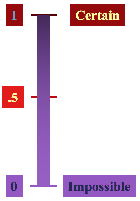
- Probability is the numeric value representing the chance/likelihood/possibility that a particular event will occur.
Some important properties of probability are:
- The value of probability lies between 0 and 1.
- Probabilities are mostly expressed as percentages.
- The sum of the probabilities of all mutually exclusive and collective exhaustive events is 1.
Probability Notation
It is very important that we learn to express probability events using a scientific notation, as we will be using these concepts extensively in all future lessons.
- P(X) denotes the probability of an event X happening.
- For example, what is the probability of getting a five when rolling a die?
- Event: getting a face with five dots
- Possible outcomes: 1, 2, 3, 4, 5, 6
denotes the probability of the event that five spots turn up when you roll a die, and X represents a variable that captures the value shown on the face when we roll a die.
It is important that we learn to use this probability notation, as we will see that it will be very useful in the course later.
We know that if we have a fair die, there is an equal chance that any one of the faces turns up. Because there are six faces on a die, we can express the probabilities as follows:
In other words, there is a 1/6th (i.e., 16.67%) chance that the face with one spot (or two or three or four or five or six) will turn up when we roll a die.
Also, remember that the cumulative probabilities of all possible outcomes should equal one. Mathematically, we can write:
A Word About Interpreting Probabilities
Suppose you toss a coin 10 times and you get seven heads and three tails. Weren’t you supposed to get five heads and five tails? What happened to the laws of probability?
We often make these kinds of mistakes when interpreting probability. Remember the assumption of probability is that you are performing the same activity many times under the same conditions. If you toss the coin 100 times instead of 10 times, you will see that you have a roughly 50-50 split between heads and tails, and the ratio of heads to tails would become increasingly equal as you toss the coin 1000, 10000, 100,000, and so on, times.
While it is easy to understand this concept with a coin toss, we still make mistakes in our everyday life. For example, what does the statement that Candidate A has a 70% chance of winning the U.S. presidential election actually mean? It means that if the elections are repeated multiple times, keeping all other factors (e.g., economy, climate, labor market, etc.) exactly the same, Candidate A will win the race about 70% of the time. This means Candidate B (U.S. presidential elections are primarily between two candidates) will win 30% of the time. Of course, elections happen only once. So, if candidate B wins, we need to understand that this was less likely to happen, not unlikely to happen.
If you remember the 2016 U.S. presidential elections, this is exactly what happened. Most polls and statistical models gave Mr. Trump a lesser likelihood to win. After the results came out, quite a few prominent news anchors said statistical models were wrong, showing a poor understanding of probability.
Probability Distribution
- Probability distribution
- Probability distribution is a table or a graph showing the different possible outcomes and their corresponding likelihood.
| X | |
|---|---|
| Head | 0.5 |
| Tail | 0.5 |
| X | |
|---|---|
| 1 | 0.167 |
| 2 | 0.167 |
| 3 | 0.167 |
| 4 | 0.167 |
| 5 | 0.167 |
| 6 | 0.167 |
| X | |
|---|---|
| Hillary Clinton wins | 0.714 |
| Donald Trump wins | 0.286 |
1 Information obtained from FiveThirtyEight: 2016 Election Forecast.
Interpreting Probability Distributions
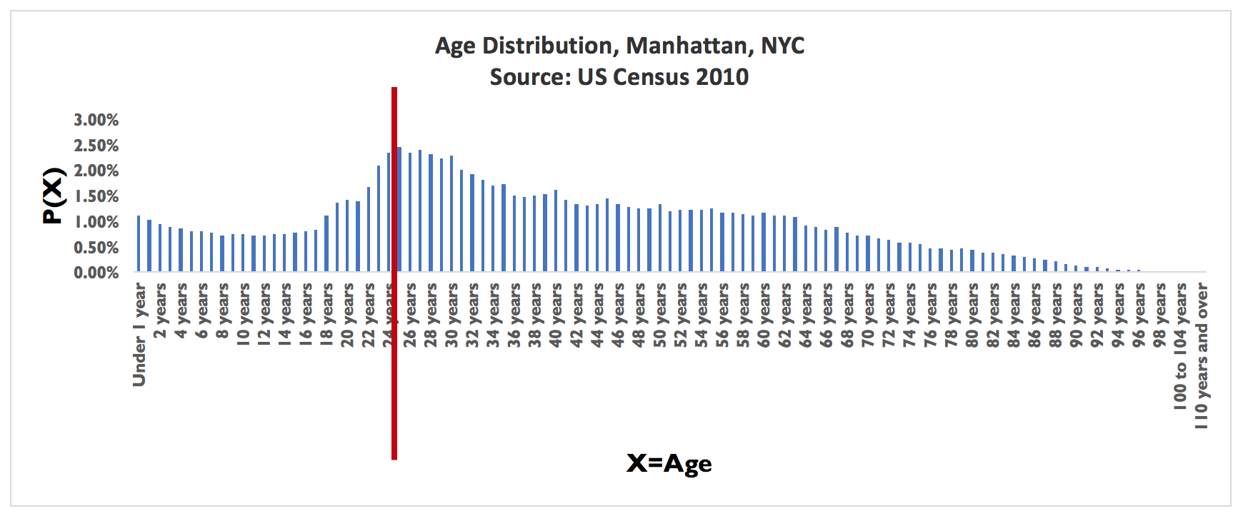
The height of each bar represents the probability of observing that particular value of the variable. For example, the height of the bar for age = 24 years represents the probability that a randomly selected Manhattan resident is 24 years old.
If we add up all the heights of the bars in Figure 2.2, it would equal 1 because we know that the cumulative probabilities equal 1.
The sum of the heights of all the bars to the left of the red line (drawn at X = 24) represent the probability that a randomly selected Manhattan resident is 24 years old or less. The sum of all the bars to the right of the red line (drawn at X = 24) represent the probability that a randomly selected Manhattan resident is more than 24 years old.
Approaches to Assigning Probabilities
Classical Approach: Based on Equally Likely Events
This approach assumes all outcomes are equally likely to occur. If an experiment has n possible outcomes, this method would assign a probability of 1/n to each outcome. It is necessary to determine the number of possible outcomes.
Experiment: Rolling a Die
- Probability that a face with five spots turns up when you roll:
- Probability that you roll four or less:
- Also note that the possibility you roll more than four:
Relative Frequency: Assigning Probabilities Based on Experimentation or Historical Data
You may remember the cumulative and relative frequencies we calculated for Google’s Project Fi customers. The relative frequencies we calculated for each category can be used as a probabilistic estimate for customer spending patterns. So, we can say there is a 6.5% chance that a new customer will spend between $30–$45, 60.5% chance that a new customer will spend $45 or less, and so on. In other words, we are using this data from a sample of 200 customers to predict the behavior of a new customer.
| Spending amount (X) in dollars | Relative frequency P(X) | Cumulative relative frequency P(X<=...) |
|---|---|---|
| 0–15 | ||
| >15–30 | ||
| >30–45 | ||
| >45–60 | ||
| >60–75 | ||
| >75–90 | ||
| >90–105 | ||
| >105–120 |
Probability a new customer spends:
- Between $30–$45
- $45 or less:
- More than $45 :
The same information can also be displayed in a chart:
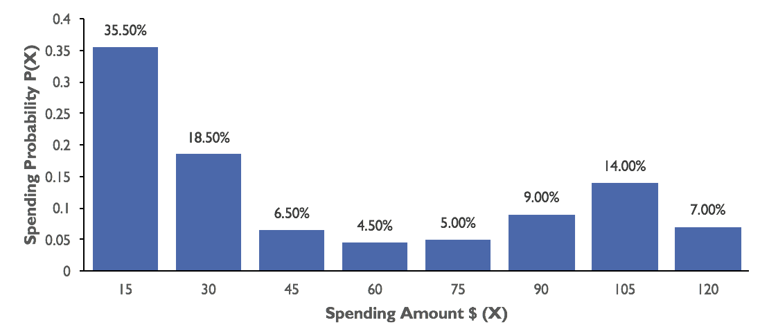
Figure 2.3. Distribution of Customer's Monthly Phone Bill
Example: What Is the Probability That a Family in Your County Has an Income > 60,000?
- Last census data shows that there were 54,345 households in your county, of which 31,496 had a income above 60K
- Sales Management Magazine reports 55,100 households, with 32,047 having income > 60K
Subjective Approach: Assigning Probabilities Based on the Assignor’s (Subjective) Judgment
In the subjective approach, we define probability as the degree of belief that we hold in the occurrence of an event.
For example, based on historical performance and current market conditions, there is a 75% chance that stock price will go up in the next quarter.
Subjective probabilities have personal biases and may vary widely from person to person.
Interpreting Probability
No matter which method is used to assign probabilities, all will be interpreted in the relative frequency approach.
For example, a government lottery game where one number (of 49) is selected. The classical approach would predict the probability for any one number being picked . We interpret this to mean that in the long run each number will be picked about 2.04% of the time.
Opening Case: Inventory Management
Inventory Management
Suppose that at a gas station, the daily demand for regular gasoline is normally distributed with a mean of 1,000 gallons and a standard deviation of 100 gallons. The station manager has just opened the station for business and notes that there is exactly 1,100 gallons of regular gasoline in storage. The manager needs help with the following:
- Issue 1: The next delivery is scheduled for later today at the close of business. The manager would like to know the probability that he will have enough regular gasoline to satisfy today’s demands.
- Issue 2: The owner wants to know how much stock he must maintain if he wants to meet demand at least 95% of the time.
Note that we have used the term "normal distribution" to describe the demand for gasoline; perhaps you have heard the term before. What does the term normal distribution mean?
Normal distribution is one of the most important probability distributions in decision-making. Many continuous variables in everyday business (e.g., age, height, income, demand, IQ, time taken to answer a customer call, etc.) follow this distribution. In the following material, we will learn about the properties of normal distribution and how that helps in decision-making.
Normal Distribution
The normal distribution is a continuous probability distribution. In a continuous probability distribution, a continuous random variable can assume an uncountable number of possible values. Some examples are time, height, weight, salary, and IQ.

Figure 2.5. Shape of a Normal Distribution
A normal distribution
- is bell-shaped;
- is symmetric around the mean; and
- has the same mean, median, and mode.
The variable () can take any value between. The mean ( ) and standard deviation ( ) of the normal distribution tell us the shape of a normally distributed curve. As long as we know these two, we can use the values to compute probability that the variable will be above or below a certain value. We will discuss this shortly. First, let's see which variables are normally distributed.
When Is the Normal Distribution Applicable?
A bell-shaped histogram usually shows up when variation in the data is primarily caused by small variations in a large number of independently operating contributing sources of variation. Here are a few examples:
- yearly sales figures of Cheerios or diapers,
- IQ,
- height,
- weight, and
- student scores.
The following possibly will not be represented by normal curve:
- weekly sales of branded material (big variations may be caused by advertising, holiday season, etc.)
- home values (big variations are caused by location, square footage, number of bedrooms)
Interpreting the Normal Distribution
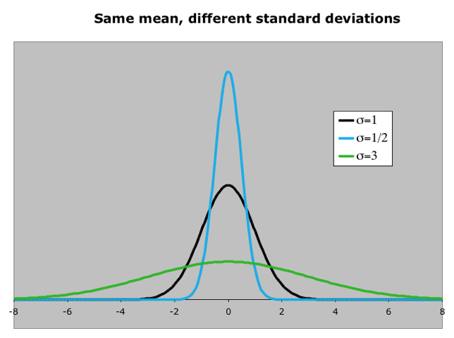
Changes in the Mean and Standard Deviation
As mentioned earlier, the normal distribution is described by two parameters, its mean and its standard deviation Increasing the mean shifts the curve to the right (see Figure 2.6) while increasing the standard deviation “flattens” the curve (see Figure 2.7). The first figure shows what happens when the mean changes. The second figure shows what happens when the standard deviation changes.

Area Under the Curve
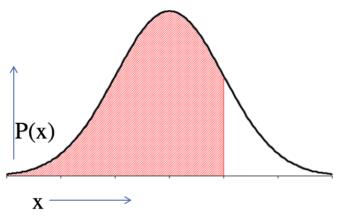
Figure 2.8. Interpreting the Area Under a Normal Distribution
A normal distribution is essentially a histogram, where the horizontal axis represents the value of the variable and the vertical axis represents the probability (i.e., the relative percentage) of finding that value (imagine that you keep reducing the bin/class width of a histogram such that the individual bars become closely packed thin slices).
Now remember from our discussion on probability that the sum of all the individual probabilities adds up to 1. So the total area under the normal distribution curve is 1. It represents the probability that the variable falls within the range to . The shaded area in the adjoining figure represents the probability that the variable is less than or equal to a particular value. The white area represents the probability that the variable is greater than or equal to a particular value.
A normal random variable can have an infinite number of values, so the probability of each individual value is virtually 0. Thus, we can determine the probability of a range of values only.
For example, with a discrete random variable like tossing a die, it is meaningful to talk about the chance that we will observe 5 when rolling the die. However, in a continuous setting (e.g., with time as a random variable), the probability that the random variable of interest, say task length, will take exactly 5 minutes is infinitesimally small (we can slice up time in nanoseconds or less), hence . It is only meaningful to talk about .
Using the Normal Curve in Inventory Management
Let's return to the first case and see how you can use normal probabilities to help the gas station owner make his decisions.
Inventory Management Issue 1: Find Probability (P)
The demand is normally distributed with mean and standard deviation . You want to find the probability
Graphically, you want to calculate the area of the shaded region. You can use Excel formulas to find the value of
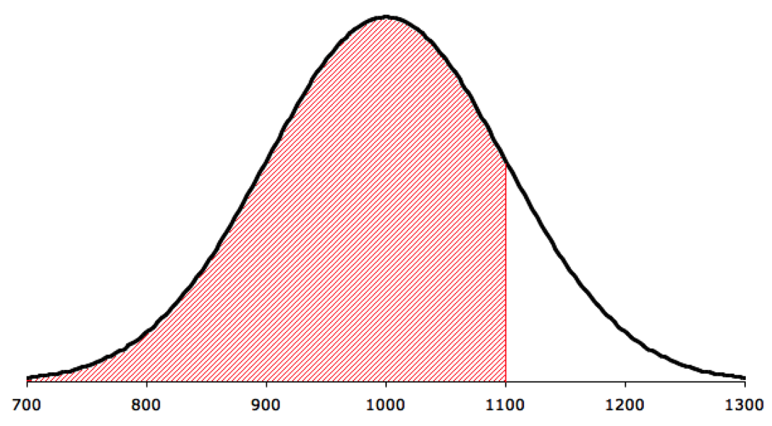
Use the NORM.DIST function to compute cumulative normal probability The function takes the following form:
You know that so the Excel formula should be entered as follows:
You will get 0.841345 as the answer.
- Therefore, there is an 84% chance that the gas station will not run out of gas today.
- Alternatively, 84% of the days, the demand is 1,100 gallons or less.
*Remember, always set Cumulative = TRUE with normal distribution. Because the normal curve represents a continuous variable, the probability that demand will be exactly 1,100 gallons is very small. We can only predict the probability of demand being less than or equal to 1,100 gallons.
Inventory Management Issue 2: Using Probability to Find Variable Values
The owner wants to know the stock level that he has to maintain if he wants to meet demand at least 95% of the time. Graphically, you want the area of the shaded portion to be 0.95, so we would like to know at what value of x (inventory level) the area on its left-hand side will be 0.95. In operations, this is known as the safety stock.
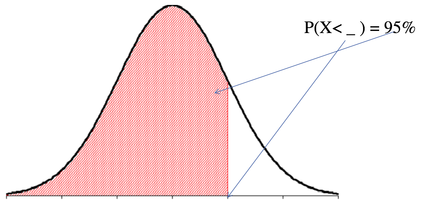
In this case, you will the NORM.INV function on Excel. The function takes the following form:
, so the Excel formula should be entered as follows
; you will get 1164.48 as the answer.
- Therefore, if the gas station keeps 1,165 gallons of gas, 95% of the time it will not run out of stock.
- Alternatively, 95% of the time, the demand is 1,165 gallons or less.
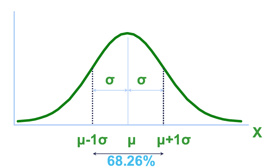
Empirical Rule: Normally Distributed Variables
For any normal distribution,
encloses about 68.26% of the data.
covers about 95.44% of the data.
covers about 99.73% of the data.
covers about 99.99% of the data.
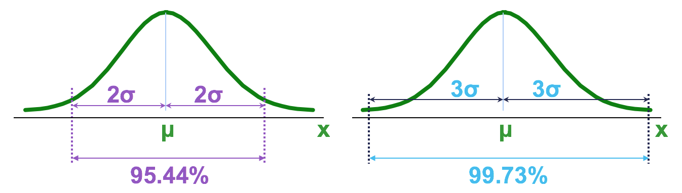
Empirical Rule: Applied to the Inventory Management Example
Remember the example where daily demand for gasoline at a pump is distributed normally with mean 1,000 gallons and standard deviation 100 gallons.
- 68.26% of the times demand is between (1,000 - 100) = 900 and (1,000 + 100) = 1,100 gallons
- 95.44% of the times demand is between (1,000 - 2*100) = 800 and (1,000 + 2*100) = 1,200 gallons
- 99.73% of the times demand is between (1,000 - 3*100) = 700 and (1,000 + 3*100) = 1,300 gallons
Z-scores
Often, we want to compare values of a variable with respect to others. We might want to know how our IQ compares with others, where we stand on the income scale compared to the rest of the U.S. population, how an employee performs in comparison to her peers, and so on. The z-distribution or the standard normal distribution is a widely used method to judge how extreme a value is compared to the average. Now that we know the properties of normal distribution, especially the empirical rule, we will see how to use these properties to compare values on a relative scale.
-
Z-score
-
The z-score is a relative comparison of an observation and is calculated using the following formula:
where x = variable value, = population mean, and σ = population standard deviation.
The z-score is a way of measuring how unusual an observation is and is the number of standard deviations above or below the mean. A z-score of zero indicates the value is the same as the mean, whereas a positive or negative value will indicate that the value is above or below the mean respectively. Let's illustrate with the following example.
Z-scores: Comparing Performance
The table below provides your performance and the class performance in two exams. On which exam did you do better?
| Class average | Class standard deviation | Your score | |
|---|---|---|---|
| Exam 1 | 50 | 10 | 60 |
| Exam 2 | 65 | 15 | 70 |
In this example, we can calculate your score in terms of z-scores.
| Exam 1 | Exam 2 | |
|---|---|---|
| Your score | ||
| Average | ||
| Standard deviation | ||
| Your score in standard units |
You scored 1 standard deviation above average in the first exam and 0.33 standard deviation above average in the second exam. So, your performance was better in the first exam although the absolute score is higher in the second one.
Interesting Fact: Einstein's IQ
IQ Scores: Mean (µ: 100; Standard Deviation
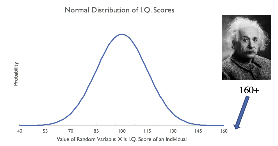
Z-score of Einstein's IQ
How extreme is z = 4 (i.e., a score 4 standard deviations above the mean)? We will see shortly.
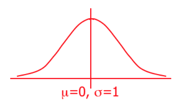
Standard Normal (z) Distribution
A normal distribution whose mean is zero and standard deviation is 1 is called the standard normal distribution.
Any normal distribution can be converted to a standard normal distribution with simple algebra. This makes calculations much easier.
Calculating in Standard Units
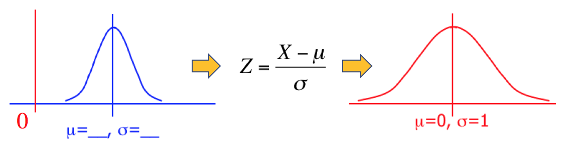
Figure 2.14. Converting a Variable (X) to the Standard Normal (Z)
Calculating Score From Standard Units
Conversely, if you know your score in standard units, you can always work backward to calculate your actual score.
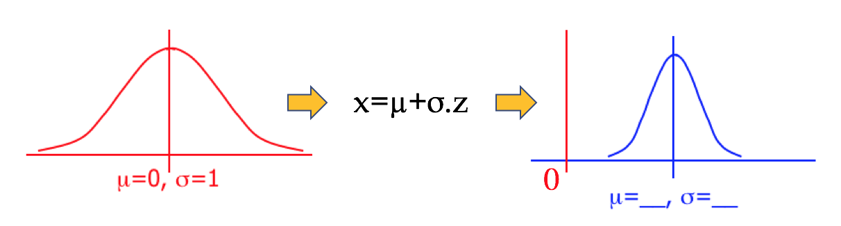
Figure 2.15. Converting the Z-score to a Variable Value (X)
Remember: Use the + sign when calculating scores that are above average.
Use the – sign for scores below average.
What is the point of using the z-score, you ask? Well, because the z is distributed with mean 0 and a standard deviation of 1, it makes calculations easier. Let’s see how we could have solved the inventory management problem discussed earlier using the z-distribution.
Inventory Management Example With Standard Units (Z)
Remember the example where daily demand for gasoline at a pump is distributed normally with mean 1,000 gallons and standard deviation 100 gallons.
If the demand on a certain day is 1,100 gallons, the Z value for X = 1,100 is
This says that X = 1,100 is one standard deviation (1 increment of 100 units) above the mean of 1,000 gallons.
Task
In the inventory management example, calculate the demand level that is
- 2 standard deviations above average
- 1 standard deviation below average
Answers
What Good Is This Information?
As we will soon see, we can very quickly convert that to a probability value. In other words, we will know what the chance is of observing a demand that is 2 standard deviations above average.
Using Standard Units (Z values)
1. What is the probability that demand is 1,200 gallons?
Remember, we can never know the probability that demand is exactly 1,200 gallons. However, we can calculate the probability that demand is less than or equal to 1,200 gallons.
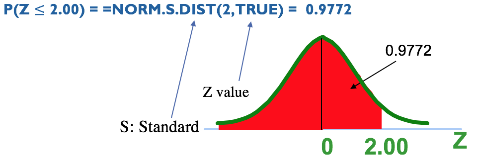
There is a 97.72% chance that demand is 1,200 gallons or less. In other words, there is only 1 – 0.9772 = 0.0227 = 2.27% chance that demand will be more than 1,200 gallons on a given day.
2. What is the probability that demand is 900 gallons?
P ( X ≤ 900 ) = NORM.DIST ( 900 , 1000 , 100 , TRUE ) = 0.1586
P ( Z ≤ -1.00 ) = NORM.S.DIST ( -1 , TRUE ) = 0.1586
There is a 15.86% chance that demand is 900 gallons or less. In other words, there is 1 – 0.1586 = 0.0227 = 84.13% chance that demand will be more than 900 gallons on a given day.
The Advantage of Using Z Over X
remains the same, no matter what the mean and standard deviation of your variable X. Take, for example, the hybrid car you bought in one of the previous examples. The car’s average mileage is 70 mpg with a standard deviation of 4 mpg. In this case, 2 standard deviation above average (i.e., Z = 2) corresponds to X = 70 + 2*4 = 78 mpg. Because you already know that , if your new car gives you 78 mpg or higher, consider yourself very lucky, since only 2.27% of those cars give that kind of mileage. Similarly, some observations falling one standard deviation below the average (z = -1) imply that only 15.86% of the values fall below that level. So, if this is the performance of the car you want to buy, you may want to rethink that decision.
In a nutshell, if we know the z-score of a variable, we know how extreme (or not) that value is.
Finding Values of
Because Z is a standard curve, often we’re asked to find some value of Z for a given probability. In other words, given an area α (i.e., probability) under the curve, what is the corresponding value of on the horizontal axis that gives us this area?
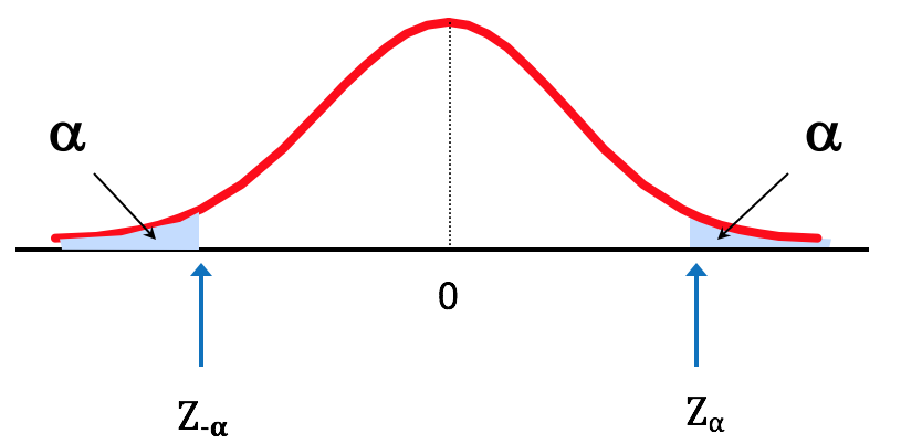
Figure 2.16. Finding the Z-score for a Given Probability
Let's consider how this is used in the examples we have seen before.
What Is the 95th Percentile Score for IQ?
Sometimes, we are interested in knowing percentile scores (e.g., your GMAT scores). A 95-percentile score (or the top 5th percentile score) implies that out of 100, only 5 score above this score and 95 score below this score.
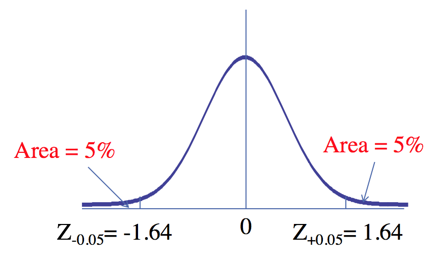
We write this as . What is the value of Z for which only 5% of all values are higher than Z?
In this case:
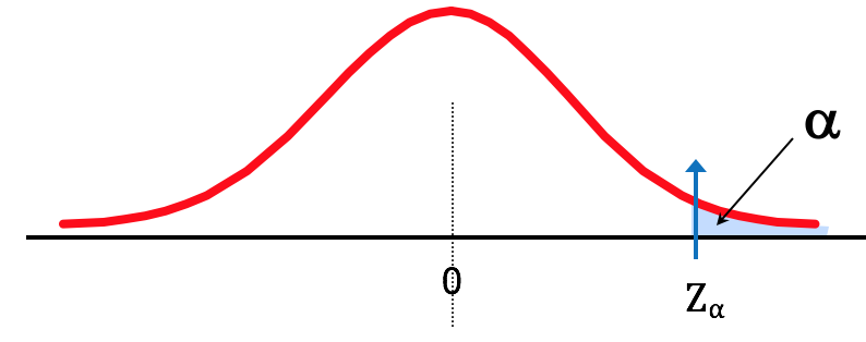
Figure 2.17. What Is the 95th Percentile IQ Score? (α = 0.05)
In Excel, we use the function NORM.S.INV (p); p is the white portion of the curve.
Note the "+" sign in . This signifies that we are talking about the top 5 percentile. will signify the bottom 5th percentile.
If IQ is distributed with a mean 100 and standard deviation 15, the 95th percentile (or top 5 percentile score) is
100 + 15*1.644854 = 124.6728
For example:
Why Learn All These Formulas?
As you will soon see in the next lessons, knowing the z-distribution helps immensely in statistical inferencing. We can always convert an observation (i.e., the value of a variable) into a z-score to tell us how many standard deviations above or below the mean that observation is. More importantly, we can also calculate how extreme the value of a variable needs to be to satisfy a certain probability.
Concept in Action: Application of Normal and Standard Normal Distributions (Z)
6
Perhaps you have heard about the term Six-Sigma. It is used extensively in quality control. Broadly speaking, Six-Sigma refers to the set of business process management techniques aimed at reducing defects (going outside specification limits). Some examples of specification limits in business include:
- All calls in a call center should be answered within 3 minutes.
- Patients in a hospital’s ED should not wait more than 45 minutes.
- All one-liter soda bottles should be filled within 0.995 liter to 1.005 liter.
Having a Six-Sigma process implies that the limits of the specifications are set such that they are six standard deviations (and hence Six-Sigma) away from the mean, making it very unlikely that the process will produce something beyond these limits.
For example, in a plant that fills one-liter soda bottles, the average amount of liquid in a bottle should be one liter. If our specification limits are 0.995 liter and 1.05 liters, then the allowed standard deviation of the process = (1 – 0.995)/6 = 0.005/6 = 0.0008333 liters. Seen from another perspective, Six-Sigma is a process of reducing variability in business processes.
Control Charts
Another use of the z distribution and the property of the standard normal curve is in operations management to test whether a process is stable. Remember the empirical rule that in a normal distribution, roughly 68% of all values fall within ±1 standard deviation (), 95% of all values fall within ±2 standard deviation (), and 99% fall within .
Control charts (an example is shown in Figure 2.19), are a major part of statistical process control (SPC). They are used for examining process quality and stability. In a control chart, horizontal markers show the process average and points 1, 2, and 3 standard deviations above and below the mean. Data points are continuously collected and plotted on the chart showing their position relative to the expected process average. If the process is stable, then we would see variations that are only due to natural randomness. So, we can expect about 68% of all the observations to fall within ± 1 standard deviation of the process mean. If there are too many points that are outside ±1σ, it is a signal to start investigating the process because it may be indicative of some non-random systematic problems. An observation beyond ±3σ may be indicative of a severe problem.
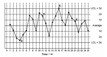
Figure 2.19. Control Chart Example
Let's look at an example. Consider that in a hospital’s emergency room (ER), the average time for a (non-severe) patient to see a clinician is 45 minutes with a standard deviation of 8 minutes. The ER admins take random observations for a month and see that 40% of such non-severe patients took more than 53 minutes to be seen by a clinician. This is certainly an indication of an underlying problem since she would expect roughly 68% of all such non-severe patients to be seen within 37 minutes (= 45 − 8) and 53 (= 45 + 8) minutes. Of the rest of the 32% (= 100% − 68%), half (i.e., 16%) should be above 53 minutes, and the other half (16%) should be below 37 minutes. That she has 40% of all patients (instead of the expected 16%) taking more than 53 minutes is certainly a red flag.
Lesson 2 Summary
- A probability distribution is a chart or a graph that shows the different possible values of the variable of interest (e.g., age, income, salary, sales, inventory level, number of calls coming in a call center, etc.) and the probability of observing that particular value.
- Probability distributions are calculated from relative frequencies. In a probability distribution, the sum of all probabilities equals 1.
- If the probability distribution is displayed as a bar graph or a solid graph (for continuous variables), the area under the curve represents the possibility of observing all outcomes and thus equals 1.
- The area on the left-hand side of a line, drawn vertically through the probability distribution, represents the probability of observing all outcomes up to the point, where the line is drawn.
- The area on the right-hand side of a line, drawn vertically through the probability distribution, represents the probability of observing all outcomes beyond the point, , where the line is drawn
- The normal distribution is a continuous probability distribution. Many variables in our daily and business lives roughly follow the normal distribution. Examples may include, but are not limited to height, weight, IQ, call durations (for one specific type of call) at a call center, height/weight/width/length (i.e., the specification parameters) of a product in a production line, number of chips in a bag, the time taken for a routine doctor visit, and so on.
- Although normal distributions are quite frequent, we often make a severe mistake in inference when we apply normal distribution formulas in scenarios where the underlying variable is not normally distributed. To avoid this mistake, look for
- small sample size,
- non-random sample, and
- infrequent large spikes.
- Although normal distributions are quite frequent, we often make a severe mistake in inference when we apply normal distribution formulas in scenarios where the underlying variable is not normally distributed. To avoid this mistake, look for
-
Template to calculate probabilities and variable values based on the normal and z-distributions.