Lesson 2: Frequency Distributions and Central Tendency (Printer Friendly Format)
page 1 of 6
Lesson 2: Frequency Distributions and Central Tendency
Introduction
In this lesson you will encounter the concept of a distribution for the first time. A distribution simply arises due to variations in performance. Such variations can be between individuals, differences within individuals over time, or they can even be variations in the size of CDs made by a particular machine. The concept of a distribution will come back throughout the course in different forms.
You will also learn about measures of central tendency. These measures, such as the average score of people on some test, provide a useful measure of behavior across people. Of course people differ from one another, but for many types of behavior people also are remarkably similar. A basic assumption of much psychological research is that the way in which behavior is controlled in one individual will be similar to the way in which behavior is controlled in another individual. By taking the average behavior of many people, one can thus study how most people control certain behaviors. Let’s get started!
Learning objectives:
( These will need to be changed to objectives that describe what students will be able to do by the end of the lesson. For example: At the end of Lesson 2 students should be able to:
1) Describe how frequency distributions and central tendency are used as descriptive statistica techniques.
- Learn about frequency distributions and central tendency as descriptive statistical techniques.
- Learn how to display frequency distributions as tables and graphs. Such tables include both regular and grouped frequency tables, and such graphs include bar graphs, histograms, and polygons.
- Learn about three different measures of central tendency, the mean, the median, and the mode. You will also learn about their relation to the shape of distributions.
page 2 of 6
Frequency Distribution Tables
After collecting data for an experiment, a researcher would first want to organize the data in such a way that it is possible to get a general feel for the results. Descriptive statistical techniques are ideal for this purpose, and all the techniques for displaying data in graphs and tables are examples of such techniques.
To get a sense of the data, a researcher may first want to generate a frequency distribution of the data. A frequency distribution is an organized tabulation showing exactly how many individuals (or units of measurement if the measure does not concern individuals) are located in each category on the scale of measurement. A frequency distribution contains the entire set of scores, and allows one to compare each score in the set to the rest of the set of scores.
A frequency distribution table is a table that displays all the scores in the set of scores, and their frequency (how often they occurred). Such a table consists of at least two columns, one listing the categories on the scale of measurement (X) and another listing their respective frequencies (f). In the X column, values are listed from highest to lowest without skipping any. In the frequency column, counts for each X are displayed. For example, if one of the scores in the set is X = 5, and three people had a score of 5, then the value f = 3 would go in the frequency column. The sum of the values in the frequency column should always equal the total number of scores in the entire set of scores (N). A third column can be included that displays the proportion (p), the value for f in the frequency column divided by the total number of values N. Thus, p = f/N. Proportions are always between 0 and 1. The sum of the p column should always equal 1. A fourth column could be included to show the percentage for each value of X. You calculate the percentage for each value of X by multiplying the proportion p by 100. The sum of the percentage column is always 100%, with the percentage for each X being between 0% and 100%.
Example 1:
A developmental psychologist is interested in determining how many minutes it takes children to complete reading a booklet. To do so, she asks ten children to read the booklet, and records the following scores:
1, 3, 1, 1, 2, 1, 2, 1, 1, 2
The following regular frequency distribution table displays these scores.
X |
f |
p = f/N |
Percentage = p x 100 |
1 |
6 |
0.6 |
60% |
2 |
3 |
0.3 |
30% |
3 |
1 |
0.1 |
10% |
In this example, N = 10, the sum of p is 1.0, and the sum of the percentages is 100%. Each square with a number in this table is called a cell.
If there are too many values for X to display them all separately, a grouped frequency table is used. In this table, the X column lists groups of scores, called class intervals. These intervals all have the same width. Each interval begins with a value that is a multiple of the interval width. The interval width should be selected in such a way that the resulting table has no more than approximately ten intervals, and no less than four.
page 3 of 6
Frequency Distribution Table Examples Continued
Example 2:
In a second test, the same psychologist wonders how long it takes 20 children to color a set of drawings. She now records the following scores in minutes:
31, 43, 36, 29, 41, 40, 33, 37, 28, 39, 30, 44, 35, 28, 40, 39, 32, 36, 27, 38
The following grouped frequency distribution table displays these scores.
The following grouped frequency distribution table displays these scores.
X |
f |
p = f/N |
Percentage = p x 100 |
25-29 |
4 |
0.2 |
20% |
30-34 |
4 |
0.2 |
20% |
35-39 |
7 |
0.35 |
35% |
40-44 |
5 |
0.25 |
25% |
N = 20, the sum of p is 1.0, and the sum of the percentages is 100% in this example.
For these same data, the following grouped frequency table with smaller intervals would also be acceptable:
X |
f |
p = f/N |
Percentage = p x 100 |
26-27 |
1 |
0.05 |
5% |
28-29 |
3 |
0.15 |
15% |
30-31 |
2 |
0.1 |
10% |
32-33 |
2 |
0.1 |
10% |
34-35 |
1 |
0.05 |
5% |
36-37 |
3 |
0.15 |
15% |
38-39 |
3 |
0.15 |
15% |
40-41 |
3 |
0.15 |
15% |
42-43 |
1 |
0.05 |
5% |
44-45 |
1 |
0.05 |
5% |
page 4 of 6
Frequency Distribution Graphs
In a frequency distribution graph, the score categories (X values) are listed on the x-axis (also called the abscissa), and the frequencies are listed on the y-axis (the ordinate). For scores that fall on an interval or ratio scale, a histogram or a polygon graph should be used. In a histogram, a bar is centered above each score (or interval) so that the height corresponds to the frequency of that score or interval and the width corresponds to the real limits of the score or interval. In a polygon, a dot is centered above each score so that the height of the dot corresponds to the frequency of the X value, and straight lines then connect the dots. At the ends, a line is drawn from the first X value with a frequency greater than zero to the first preceding or following X value for which the frequency is zero, so that the graph returns to zero at both ends.
For scores that fall on a nominal or ordinal scale, a bar graph should be used to display the data. A bar graph is similar to a histogram except that the width of the bars does not correspond to the real limits. Thus, the heights of bars correspond to the frequencies of the X values, but there is a gap between adjacent bars to indicate that the scale of measurement is not continuous.
Often, populations of interest are too large to know the exact frequencies of any of the specific categories (X values). In such a case, population distributions can be shown using relative frequency instead of the absolute number of individuals per category. If the scores are measured on an interval or ratio scale, the histogram and/or polygon used to display the data presents a smooth curve between the values rather than a jagged pattern, to reflect the fact that the distribution is not showing exact frequencies for each category but only estimations.
Central tendency is a term that refers to a set of measures that capture accurately the center of a distribution. As such, these measures provide information about an entire set of scores, condensed into one value. There are three different measures of central tendency that we will consider in this course, the mean, the median, and the mode. It is important to realize that although each of these measures concerns central tendency, they often take on different values for a given set of scores. This is because each of these measures is sensitive to aspects of the distribution, such as its shape.
page 5 of 6
Central Tendency Measures
The mean is the most common measure of central tendency, and it will be an important concept throughout the course. Computing the mean requires scores that are numerical values measured on an interval or ratio scale. The mean is calculated by taking the sum of all the scores, and then by dividing this sum by the number of scores in the in set.
For sample data the mean is:
M = ΣX/n (n being the sample size)
For population data the mean is:
μ = ΣX/N (N being the size of the population)
Conceptually, you can think of the mean as the amount that every individual would get if the total (ΣX) is divided equally between all the individuals (n or N, depending on whether it is a sample of people or the whole population). The mean is the balance point of the distribution, with equal ‘weight’ to each side of it.
Because the mean is based on every score in the set of scores, changing a score will also change the mean. Similarly, adding or removing scores will also almost always change the mean, unless the score that is added or remove is exactly equal to the mean.
Although the mean is the most commonly used measure of central tendency, there are situations in which the mean does not provide an accurate reflection of the distribution as a whole. We will come back to this point after introducing the other two measures of central tendency.
A second measure of central tendency is the median. The median is the value that corresponds to the exact midpoint of all the values. Thus, if you have a list of scores and order them going from lowest to highest, the median would be the score that is the midpoint of this list. The median divides the set of scores in such a way that 50% of the scores is smaller or equal to the median, and 50% is greater or equal to the median. Computing the median requires the scores to be put in rank order, and therefore the scores must come from an interval, ordinal, or ratio scale. Usually, the median can be found by the following counting procedure:
- With an odd number of scores, list the scores in order. The median is the middle value in the list of scores.
- With an even number of scores, list the scores in order. The median is the halfway between the two middle values in the list of scores. To get the halfway point, sum the two scores in the middle and divide the sum by 2.
A third measure of central tendency is the mode. The mode is defined as the most frequently occurring score in the distribution of scores. In a frequency distribution graph, the mode corresponds to the highest point on the graph. The mode can be determined for any scale, be it nominal, ordinal, interval, or ratio. The primary value of the mode is that it is the only measure of central tendency that can be used for measurements on a nominal scale.
Unlike the other two measures, a distribution can have more than one mode. If there is only one prominent peak in the distribution, the shape of the distribution is unimodal. If there are two prominent peaks, the distribution is called bimodal.
page 6 of 6
The Shape of a Distribution
The shape of a distribution of scores is usually described as either symmetric, meaning that it is similar on both sides of the center, or skewed, meaning that the values are more spread out on one side of the center than on the other. If it is skewed to the right, the higher values (toward the right on a number line) are more spread out than the lower values. If it is skewed to the left, the lower values (toward the left on a number line) are more spread out than the higher values. A symmetric dataset may be bell-shaped or another symmetric shape. Figures 1, 2 and 3 show examples of three different shapes.
Figure 1: A symmetric shape
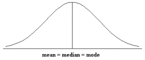
Figure 2: Data skewed to the right (also called positively skewed)
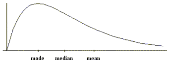
Figure 3: Data skewed to the left (also called negatively skewed)
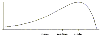
As these three figures indicate, the mean can be quite strongly affected by the shape of the distribution and the presence of extreme scores. The median and mode are less strongly affected by these factors.
Lesson 2 Assignments:
1. Complete Homework Chapter 2
2. Complete Evaluation exercises Chapter 2 (possible direct link to homework assignments if we are able to do this with Web Assign)