Supply

The Supply Curve: The Relationship Between Price and Quantity Supplied

• The definition of quantity supplied: the amount of a good that sellers are willing and able to sell.
  • Quantity supplied is positively related to price. This implies that the supply curve will be upward sloping.
  • The definition of the law of supply: the claim that, other things equal, the quantity supplied of a good rises when the price of the good rises.
• The definition of supply schedule: a table that shows the relationship between the price of a good and the quantity supplied.
• The definition of supply curve: a graph of the relationship between the price of a good and the quantity supplied.

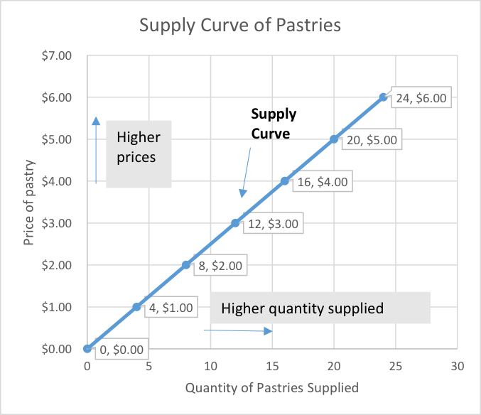
Example of Supply Schedule

Assume that you run a bakery shop and sell pastries. In the following table, you can find the supply schedule of your pastries. Table 1.2 shows how many pastries you are willing to sell at different price levels.

Table 1.2. Supply Schedule

Price of pastry	Quantity of pastries supplied
$0.00	0
$1.00	4
$2.00	8
$3.00	12
$4.00	16
$5.00	20
$6.00	24

Example of Supply Curve

We draw the supply curve by plotting each of the points from the supply schedule like an (x, y) coordinate system (see Figure 1.3).

Market Supply Versus Individual Supply

• The market supply curve is obtained from individual supply curves. We add up individual supply curves horizontally at each price.
• The market supply curve shows how the total quantity supplied varies as the price of the good varies.

Shifts in the Supply Curve

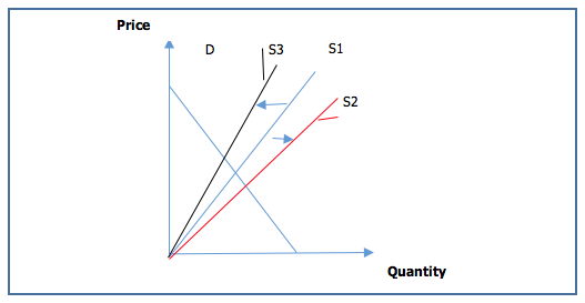
First, please note the difference between a change in price (which causes a movement along the supply curve) and a change in another determinant (which shifts the supply curve). If the price of the product is the only changing determinant, this will lead to change in quantity supplied. In Figure 1.4, it is represented by a movement along the supply curve. If other determinants change, such as cost of production, expected profits, and so on, this will lead to a change in supply. In the figure, this is represented by shifts of the supply curve.

In Figure 1.4, assume that a market has been represented. D is the demand curve in the market and S1 (blue line) is the original supply curve. S2 (red line) represents a higher supply (S1 shifts to the right and becomes S2). S3 (black line) represents a lower supply (S1 shifts to the left and becomes S3).

• Because the market supply curve holds other things constant, the supply curve will shift if any of the following factors, such as input prices, technology, and so on, change.
  • An increase in supply is represented by a shift of the supply curve to the right.
  • A decrease in supply is represented by a shift of the supply curve to the left.
• Input prices:
  • Higher cost of production (higher wages and/or higher costs of materials) lowers supply.
  • Lower cost of production (lower wages and/or lower costs of materials) raises supply. 
• Technology: Improved technology shifts the supply curve to the right.
• Expectations: Higher expected profits raise current supply. Lower expected profits cut current supply.
• Number of sellers: A higher number of producers raises supply, and a lower number of producers lowers supply.

The Supply Function

• The supply function for Good X is a mathematical representation describing how many units will be produced at alternative prices for X, alternative input prices W, and alternative values of other variables that affect the supply for Good X.
• One simple but useful representation of a supply function is the linear supply function:

${Q_X}^s={\beta }_0+{\beta }_X{P}_X+{\beta }_{W}W+{\beta }_{\mathrm{r }}T+{\beta }_{H}H$

• Q_X^s is the number of units of Good X produced;
• P_X is the price of Good X;
• W is the price of an input, such as wages, raw materials, or capital;
• T is technologically related inputs; and
• H is the value of any other variable affecting supply.

• The signs and magnitude of the $\beta$ coefficients determine the impact of each variable on the number of units of X produced:

${Q_X}^s={\beta }_0+{\beta }_X{P}_X+{\beta }_{W}W+{\beta }_{r}T$

• For example:
  • ${\beta }_X>0$ by the law of supply. Higher prices, higher quantity supplied. ${\beta }_X=\frac{\text{Change in} {Q_X}^s}{\text{Change in} P_X}$
  • ${\beta }_W<0$ increasing input price. Higher input prices, lower quantity supplied.
  • ${\beta }_r>0$ technology lowers the cost of producing Good X. Better technology, higher quantity supplied.