Main Content
Lesson 1: Decision Making Under Uncertainty

Graphical Summaries
Graphs and charts also provide effective tools for describing data; but they are only starting points. However, they are often good complements to descriptive statistics in presentations of data analysis.
Graphing One Quantitative Variable
Two of the most commonly used graphs for one quantitative variables are the histogram and box plot. We have already learned about box plots and will now create histograms.
- Histogram
-
The histogram is one of the most important and common graphs used to display quantitative variables. A histogram is essentially a bar graph for measurement data. In a histogram, the categories are a range of numbers. Usually, each numerical category must have the same width. The heights of the bars either reflect the frequency or the relative frequency (percent) of encountering that range of numbers in the data. To create histograms, we need to understand the concept of frequencies. We will illustrate this using the following case.
Case II: Monthly Telephone Bills
Google’s Project Fi is a new wireless phone service that seamlessly switches a customer’s phone between a handful of networks—Sprint, T-Mobile, and U.S. Cellular—to get the best possible signal at any given time. It also taps into reliable public Wi-Fi networks (with its own layer of encryption in place) and uses those for calls and data whenever it can.
The marketing manager at Google wants to acquire information about the monthly bills of new subscribers in the first month after signing with the company. The company’s marketing manager surveyed 200 new subscribers wherein the first month’s bills were recorded. These data are stored in files FiMonthlyBills.xlsx (Excel) and FiMonthlyBills.sav (SPSS). The manager planned to present his findings to senior executives.
In this example, we create a frequency distribution by counting the number of observations that fall into a series of intervals, called classes.
We choose eight classes defined in such a way that each observation falls into one—and only one—class. These classes are defined as follows:
Classes
- amounts that are less than or equal to 15
- amounts that are more than 15 but less than or equal to 30
- amounts that are more than 30 but less than or equal to 45
- amounts that are more than 45 but less than or equal to 60
- amounts that are more than 60 but less than or equal to 75
- amounts that are more than 75 but less than or equal to 90
- amounts that are more than 90 but less than or equal to 105
- amounts that are more than 105 but less than or equal to 120
Frequency Distribution
- Frequency Distribution
- A frequency distribution is a tabular summary showing the frequency of observations in each of several non-overlapping (mutually exclusive) classes or cells. There can be different types of frequency distributions.
- (Observed) Frequency
- This is the actual number of occurrences in a cell.
- Relative Frequency
- This type of frequency distribution displays the fraction or proportion of observations that fall within a cell.
- Cumulative Frequency
- This type of frequency distribution displays the proportion or percentage of observations that fall below the upper limit of a cell.
So, the first task is to calculate the frequencies in each of our defined classes (0–$15, $15–$30, …). To do this, we will first create the histograms and then interpret the output.
Using Technology
 Graphing a Histogram: SPSS Instructions Cumulative and Relative Frequencies: SPSS Instructions
In general, all of the graphs in SPSS can be found by going to Graphs > Chart Builder. From there, choose the appropriate graph for the given variable you want to summarize. View the Directions on Creating Charts in SPSS for specifics.
Relative and Cumulative Relative Frequencies
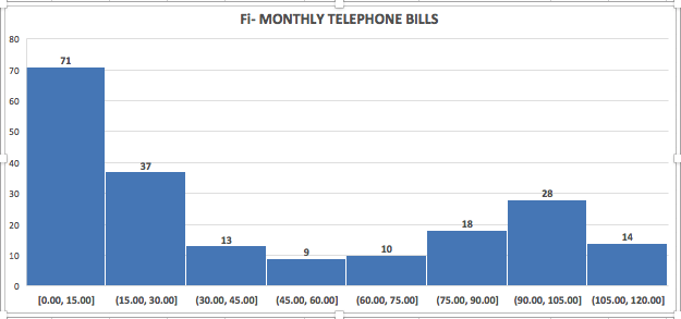
As we can see from our graphical output, 71 customer bills were in the range $0–$15, 37 customer bills were in the range $15–$30, and so on. These are the observed frequencies in each of the classes. We had a total of 200 customer data. So, the relative frequency of the spending class $0–$15 is 71/200 = 35.5%. The relative frequencies of each of the spending classes are shown in the figure below.
| Spending amount | Relative frequency |
|---|---|
| $0–$15 | 71/200 = 0.355 |
| >$15–$30 | 37/200 = 0.185 |
| >$30–$45 | 13/200 = 0.065 |
| >$45–$60 | 9/200 = 0.045 |
| >$60-$75 | 10/200 = 0.050 |
| >$75–$90 | 18/200 = 0.090 |
| >$90–$105 | 28/200 = 0.140 |
| >$105–$120 | 14/200 = 0.070 |
| Total | 200/200 = 1.0 |
The cumulative frequencies include the frequencies of all classes up to that point, as shown below.
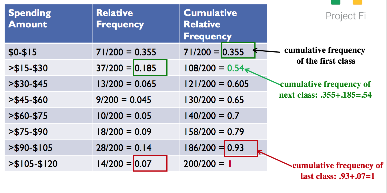
Figure 1.15. Cumulative Relative Frequencies
As we will see in Lesson 2, knowledge of histograms and frequency distributions forms the basis of understanding probability distributions.
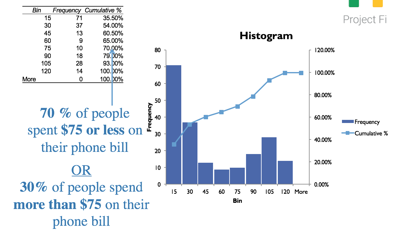
Figure 1.16. Interpreting Cumulative Relative Frequencies
You may refer to the FiMonthlyBills-Solution.xls file to see the formulas used in the example.