Main Content
Lesson 2: Distributions

Approaches to Assigning Probabilities
Classical Approach: Based on Equally Likely Events
This approach assumes all outcomes are equally likely to occur. If an experiment has n possible outcomes, this method would assign a probability of 1/n to each outcome. It is necessary to determine the number of possible outcomes.
Experiment: Rolling a Die
- Probability that a face with five spots turns up when you roll:
- Probability that you roll four or less:
- Also note that the possibility you roll more than four:
Relative Frequency: Assigning Probabilities Based on Experimentation or Historical Data
You may remember the cumulative and relative frequencies we calculated for Google’s Project Fi customers. The relative frequencies we calculated for each category can be used as a probabilistic estimate for customer spending patterns. So, we can say there is a 6.5% chance that a new customer will spend between $30–$45, 60.5% chance that a new customer will spend $45 or less, and so on. In other words, we are using this data from a sample of 200 customers to predict the behavior of a new customer.
| Spending amount (X) in dollars | Relative frequency P(X) | Cumulative relative frequency P(X<=...) |
|---|---|---|
| 0–15 | ||
| >15–30 | ||
| >30–45 | ||
| >45–60 | ||
| >60–75 | ||
| >75–90 | ||
| >90–105 | ||
| >105–120 |
Probability a new customer spends:
- Between $30–$45
- $45 or less:
- More than $45 :
The same information can also be displayed in a chart:
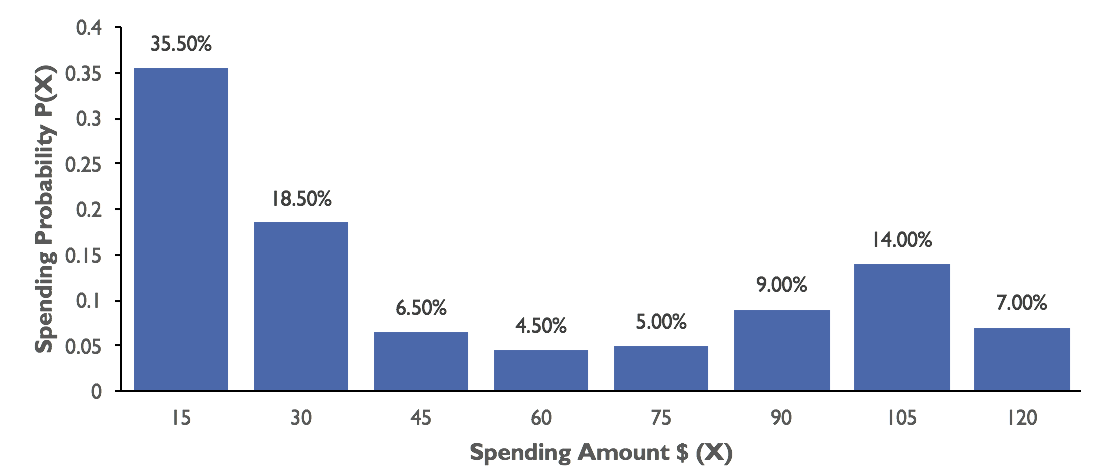
Figure 2.3. Distribution of Customer's Monthly Phone Bill
Example: What Is the Probability That a Family in Your County Has an Income > 60,000?
- Last census data shows that there were 54,345 households in your county, of which 31,496 had a income above 60K
- Sales Management Magazine reports 55,100 households, with 32,047 having income > 60K
Subjective Approach: Assigning Probabilities Based on the Assignor’s (Subjective) Judgment
In the subjective approach, we define probability as the degree of belief that we hold in the occurrence of an event.
For example, based on historical performance and current market conditions, there is a 75% chance that stock price will go up in the next quarter.
Subjective probabilities have personal biases and may vary widely from person to person.
Interpreting Probability
No matter which method is used to assign probabilities, all will be interpreted in the relative frequency approach.
For example, a government lottery game where one number (of 49) is selected. The classical approach would predict the probability for any one number being picked . We interpret this to mean that in the long run each number will be picked about 2.04% of the time.