Main Content
Lesson 2: Distributions

Concept in Action: Application of Normal and Standard Normal Distributions (Z)
6
Perhaps you have heard about the term Six-Sigma. It is used extensively in quality control. Broadly speaking, Six-Sigma refers to the set of business process management techniques aimed at reducing defects (going outside specification limits). Some examples of specification limits in business include:
- All calls in a call center should be answered within 3 minutes.
- Patients in a hospital’s ED should not wait more than 45 minutes.
- All one-liter soda bottles should be filled within 0.995 liter to 1.005 liter.
Having a Six-Sigma process implies that the limits of the specifications are set such that they are six standard deviations (and hence Six-Sigma) away from the mean, making it very unlikely that the process will produce something beyond these limits.
For example, in a plant that fills one-liter soda bottles, the average amount of liquid in a bottle should be one liter. If our specification limits are 0.995 liter and 1.05 liters, then the allowed standard deviation of the process = (1 – 0.995)/6 = 0.005/6 = 0.0008333 liters. Seen from another perspective, Six-Sigma is a process of reducing variability in business processes.
Control Charts
Another use of the z distribution and the property of the standard normal curve is in operations management to test whether a process is stable. Remember the empirical rule that in a normal distribution, roughly 68% of all values fall within ±1 standard deviation (), 95% of all values fall within ±2 standard deviation (), and 99% fall within .
Control charts (an example is shown in Figure 2.19), are a major part of statistical process control (SPC). They are used for examining process quality and stability. In a control chart, horizontal markers show the process average and points 1, 2, and 3 standard deviations above and below the mean. Data points are continuously collected and plotted on the chart showing their position relative to the expected process average. If the process is stable, then we would see variations that are only due to natural randomness. So, we can expect about 68% of all the observations to fall within ± 1 standard deviation of the process mean. If there are too many points that are outside ±1σ, it is a signal to start investigating the process because it may be indicative of some non-random systematic problems. An observation beyond ±3σ may be indicative of a severe problem.
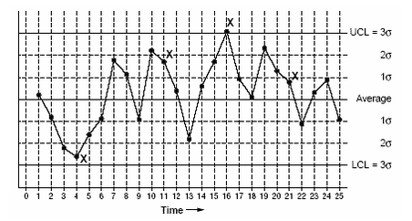
Figure 2.19. Control Chart Example
Let's look at an example. Consider that in a hospital’s emergency room (ER), the average time for a (non-severe) patient to see a clinician is 45 minutes with a standard deviation of 8 minutes. The ER admins take random observations for a month and see that 40% of such non-severe patients took more than 53 minutes to be seen by a clinician. This is certainly an indication of an underlying problem since she would expect roughly 68% of all such non-severe patients to be seen within 37 minutes (= 45 − 8) and 53 (= 45 + 8) minutes. Of the rest of the 32% (= 100% − 68%), half (i.e., 16%) should be above 53 minutes, and the other half (16%) should be below 37 minutes. That she has 40% of all patients (instead of the expected 16%) taking more than 53 minutes is certainly a red flag.