Inventory Management Example With Standard Units (Z)

Remember the example where daily demand $\left(X\right)$ for gasoline at a pump is distributed normally with mean $\left(\mu \right)$ 1,000 gallons and standard deviation $\left(\sigma \right)$ 100 gallons.

If the demand on a certain day is 1,100 gallons, the Z value for X = 1,100 is

$z=\frac{x-\mu }{\sigma }=\frac{\mathrm{1,100}-\mathrm{1,000}}{100}=1$

This says that X = 1,100 is one standard deviation (1 increment of 100 units) above the mean of 1,000 gallons.

Task

In the inventory management example, calculate the demand level that is

1. 2 standard deviations above average
2. 1 standard deviation below average

Answers

What Good Is This Information?

As we will soon see, we can very quickly convert that to a probability value. In other words, we will know what the chance is of observing a demand that is 2 standard deviations above average.

Using Standard Units (Z values)

1. What is the probability that demand is 1,200 gallons?

Remember, we can never know the probability that demand is exactly 1,200 gallons. However, we can calculate the probability that demand is less than or equal to 1,200 gallons.

$P\left(X\le 1200\right)=\text{NORM.DIST}\left(1200,1000,100,\text{TRUE}\right)=0.9772$
$P\left(Z\le 2.00\right)=\text{NORM.S.DIST}\left(2\text{, TRUE}\right)=0.9772$

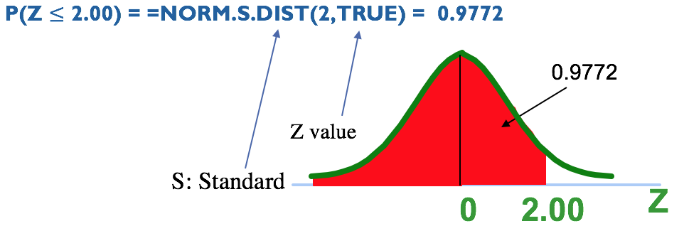
There is a 97.72% chance that demand is 1,200 gallons or less. In other words, there is only 1 – 0.9772 = 0.0227 = 2.27% chance that demand will be more than 1,200 gallons on a given day.

2. What is the probability that demand is 900 gallons?

P  (  X  ≤  900  )  =  NORM.DIST  ( 900 , 1000 , 100 , TRUE )  =  0.1586 
P  (  Z  ≤  -1.00  )  =  NORM.S.DIST  (  -1 , TRUE  )  =  0.1586

There is a 15.86% chance that demand is 900 gallons or less. In other words, there is 1 – 0.1586 = 0.0227 = 84.13% chance that demand will be more than 900 gallons on a given day.

 

The Advantage of Using Z Over X

$P\left(Z<2\right)=0.9772$ remains the same, no matter what the mean and standard deviation of your variable X. Take, for example, the hybrid car you bought in one of the previous examples. The car’s average $\left(\mu \right)$ mileage is 70 mpg with a standard deviation $\left(\sigma \right)$ of 4 mpg. In this case, 2 standard deviation above average (i.e., Z = 2) corresponds to X = 70 + 2*4 = 78 mpg. Because you already know that $P\left(Z<2\right)=0.9772$, if your new car gives you 78 mpg or higher, consider yourself very lucky, since only 2.27% of those cars give that kind of mileage. Similarly, some observations falling one standard deviation below the average (z = -1) imply that only 15.86% of the values fall below that level. So, if this is the performance of the car you want to buy, you may want to rethink that decision.

In a nutshell, if we know the z-score of a variable, we know how extreme (or not) that value is.