
Simple Averages
In simple averages, the next period's forecast is the average of all previous actual values.
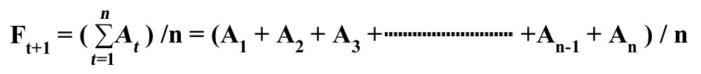
In this case, the underlying assumption is that all history has a bearing on the most recent events. The fluctuations that are seen from period to period are assumed to be merely random events that cannot be predicted with any certainty. In practice, this method will damp out all fluctuations and as the data series becomes increasingly long, it will become increasingly less sensitive to any recent movements in data. It would be most appropriate to use this approach where there are considerable random variations in the observed values but no long term evidence of either a rising or falling trend. The averaging techniques in such cases smooth out the time series as the individual high and lows cancel out each other. Consequently, the forecast value over time will become increasingly stable. The biggest disadvantage, however, is that if trend is present in the time series data, the averaging technique will lag the forecast. In other words, in the presence of an increasing trend, the use of the simple averaging technique will understate the actual value; and in the presence of a negative trend, it will overstate the actual value. Projects, however, mostly encounter situations that are not usually stable and hence this method might not be an appropriate forecasting technique for a typical project situation.