Example of Exponential Smoothing

Consider the time series with nine periods of data:

34, 38, 46, 41, 43, 48, 51, 50, 56

Use exponential smoothing to forecast the value for period 10.

Assume F₂= A₁= 34 and = 0.2.

Solution:

Using the exponential smoothing formula

New forecast = old forecast + (latest observation - old forecast),

the forecast for period 3 is given by:

F₃= F₂ + (A₂ - F₂) = 34 + 0.2(38 - 34) = 34.8

Similarly, the forecast for period 4 will be:

F₄ = F₃ + ( A₃ - F₃) = 34.8 + 0.2(46 - 34.8) = 37.04

This process can be repeated for the remaining periods to get a smoothed series given below.

34, 34.8, 37.04, 37.83, 38.87, 40.69, 42.75, 44.20, 46.56

Thus, the forecast for period 10 is given by F₁₀ = 46.56

It can be seen that this series does produce a smooth trend but it also shows a marked "lag." Sensitivity of the forecasts for the above example can be improved by changing the value of a to 0.5. In this case the smoothed series becomes:

34, 36, 41, 42, 45, 48, 49, 49.5, 52.75 and the forecast for period 10 is now given by:

F₁₀ = 52.75.

The results obtained for these different smoothing factors are shown graphically in Figure 2.1 below. See the highly damped smoothing and the considerable lag associated with the forecasts generated using = 0.2 when compared to = 0.5.

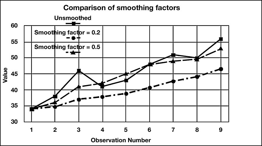
Figure 2.1 Comparison of Forecasts Generated by Different Smoothing Factors