
2.3.4 Limitations in Forecasting Using Linear Regression (continued)
There are, of course, many occasions when a simple linear model will not adequately describe the relationship between one variable and another. Unlike the linear case, there is no simple or direct method of defining the equation, although some computerized statistics packages will generate best fit curves according to a quadratic ( y=kx2 + c ) or a cubic ( y = kx3 + c ) law. Over short ranges of data where there is very little scatter, it is sometimes possible to get quite precise fits by a trial and error method, using different coefficients and taking successively higher powers of x to obtain an nth order regression. However, it must be remembered that such an empirical relationship only holds good within the range of actual data and cannot be extrapolated far beyond it.
Some curvilinear relationships can be described by the general expression:
Y - c = kxn
This expression generates a series of smooth curves with no turning points that can have a rising slope, when n is positive, or a downward slope when n is negative for x > 0. In the above expression, if we let y - c = y' , then we can transform the curvilinear equation into a straight line by taking logarithms of both sides of the above expression. Thus y' = kxn can be transformed into:
Logey' = Logek + nLogex
This relationship is most easily visualized using Log-Log graphical scales where it will be seen that a curved primary relationship can be transformed into a linear one. This is a useful method of generating an equation that will fit a series of data points and it also allows some well known curvilinear functions to be handled with greater ease. A particularly important example of the latter in engineering project work is the Learning Curve. For example, consider the two equations: y = 10x0.5 and y = 200x-0.33 . Plotted on linear scales, they appear as below.
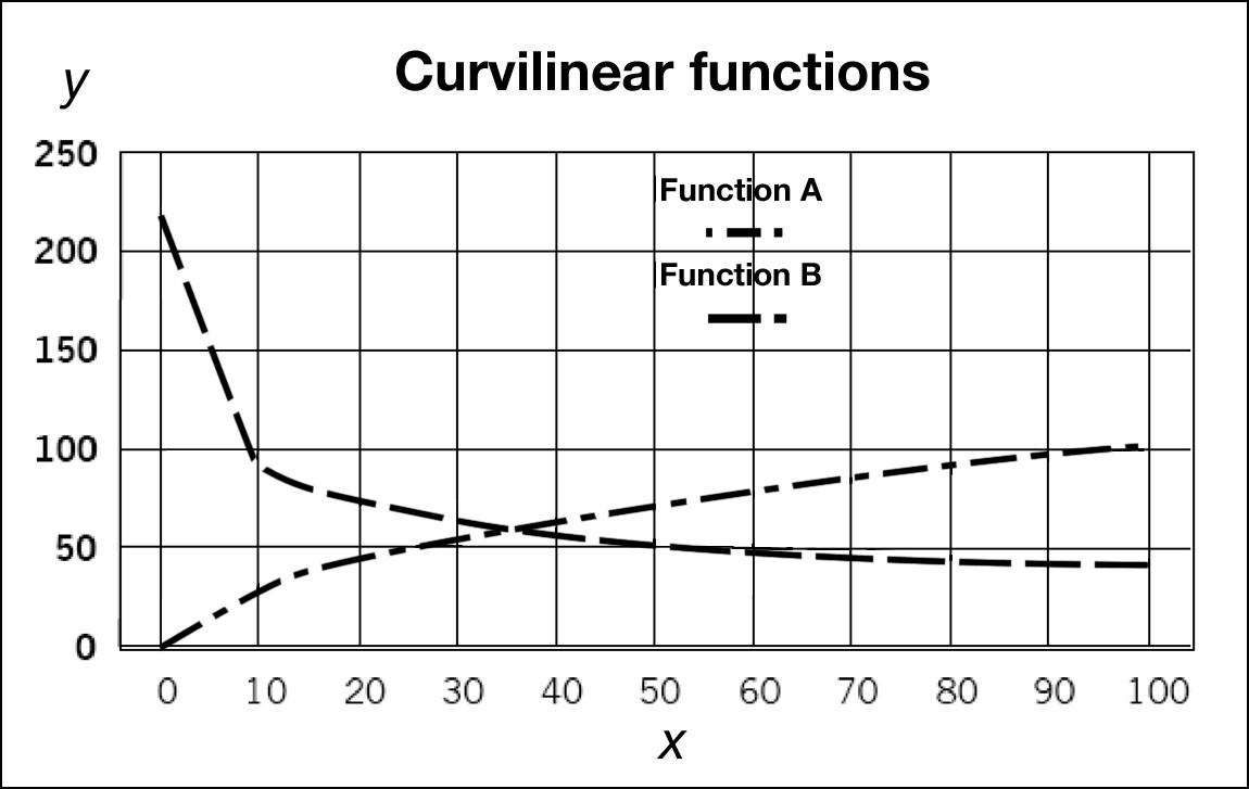
Figure 2.4 Plots of Functions (A) y = 10 x0.5 and (B) y = 200 x-0.33 on Linear Scales
Plotted on logarithmic scales, these curves now become straight lines as shown below in Figure 2.5.
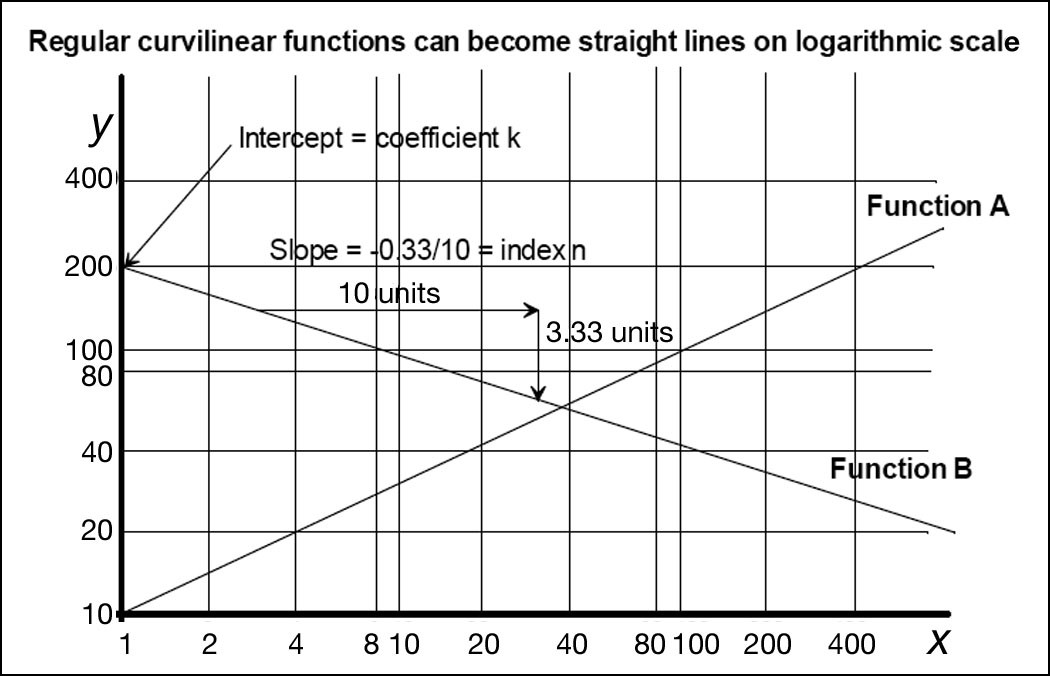
Figure 2.5 Plots of functions (A) y = 10x0.5 and (B) y = 200 x-0.33
Logarithmic plots are an extremely useful way of analyzing trends as many phenomena progress as a simple law of the form y = kxn. The rate of progress of the performance of some technologies can be clearly illustrated by linear logarithmic trends over time. Some frequency distributions can be illustrated using logarithmic plots. Once a straight line has been established, it is a simple process to compute the underlying equation. Furthermore, a straight line can be used as the basis for forecasting future values of the observed variable simply by projecting it forward. However, we must be careful about just how far ahead we can project to generate forecasts.