2.3.4 Limitations in Forecasting Using Linear Regression

For the above example, If we plot the actual y values and the forecasted values using linear regression the graph is as shown below in Figure 2.3.

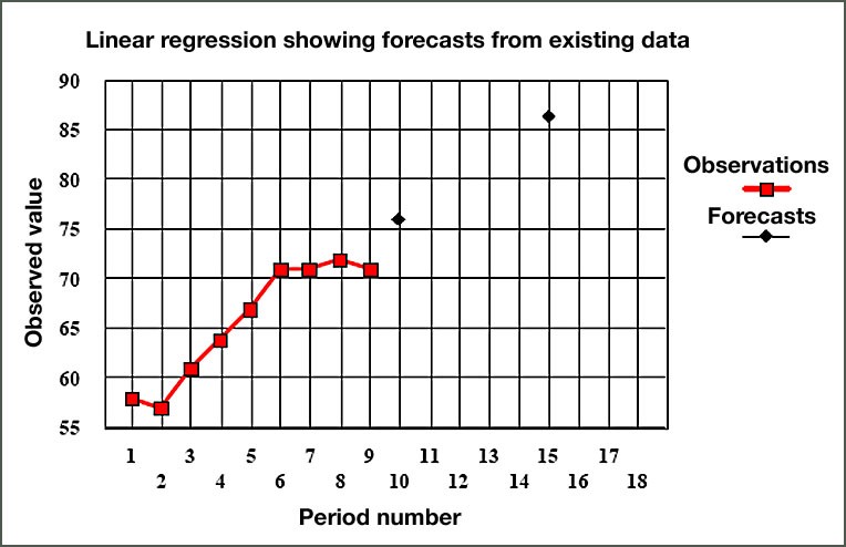
Figure 2.3 Forecasts using Linear Regression

In the above figure, notice that the forecasts using the regression equation shows a continuously rising trend. However, the pattern of actual observations, particularly over the last 4 periods, indicates a leveling off or perhaps even a down-turn. In such cases, the actual observations should, if possible, be investigated for any causes that can be discovered to account for this pattern. If there are substantial reasons for the behavior of the latest observations, these should always be taken into account when assessing the degree of credence to be placed in the regression forecast. It will also be clear from this example that the number of observations used to calculate the regression line can have a marked influence on the forecast. Where the number of observations is small, e.g., 4 or 5 values, serious errors can occur if the data happens to be behave badly.

In the example shown above, only one independent variable was considered. However, there may be occasions where several independent variables simultaneously influence the dependent variable. In such cases, an extension of linear regression technique called Multiple Linear Regression can be used. Multiple linear regression equation is of the form:

y = b₀ + b₁x₁ + b₂x₂ + b₃x₃ + .... + b_ix_i + e, where

x₁, x₂, x₃ and x_i, etc., are independent variables, and e is the error term.

b₀, b₁, b₂, b₃, and b_i, etc. are termed the regression coefficients and they represent the amount by which y changes for one increment of x_i assuming all other independent variables (x) are held constant. Students interested in learning more about this procedure should consult a statistics text. Two such texts are referenced on the final page of this lesson.