
2.3 Intermediate Term Forecasting
2.3.1 Linear Regression Analysis
One of the most useful techniques to evaluate and forecast the trend component of a time series is regression analysis. The trend component may or may not be linear. For example, the typical S-curves that we use in managing projects exhibit a non-linear trend. However, there are several project situations where the relationship of a project variable as a function of time can be assumed to have a linear trend. For example, forecasting the cost of an activity as function of time can be assumed to have a linear trend. While the assumption of linearity may not hold good in many situations over the long term, a linear relationship is often a reasonable assumption in the intermediate time frame. In such cases, linear regression analysis is a viable forecasting technique. It is also a useful methodology for determining the empirical relationship between two project variables if the underlying reasons if the relationship between those variables can be hypothesized to be approximately linear. In order to evaluate the trend component of a time series, we use linear regression analysis to develop a linear trend equation. This is the equation of a Straight Line is given by
yt = a + bt + e
Where b is the slope (gradient) of the line and a is the intercept with the y axis at t = 0, y t is the value of the project variable (for which we desire a forecast) at time period t and e is the forecast error.
The technique of linear regression analysis involves determining the values for "a" and "b" for a given data set. From a graphical perspective, the technique involves drawing a straight line that best fits the scatter of observed values that have been plotted over time (see Figure 2.1 below). "Best fit" means the difference between the actual Y-values and predicted Y-values are a minimum. However, positive differences will offset negative differences, hence we square the differences. Mathematically, the best fitting line is the one in which the sum of the squares of the deviations of all the data points from the calculated line is a minimum. In essence we are choosing a line where the scatter of the observed data about the line is at its smallest. The technique of "Least Squares Regression" minimizes this sum of the squared differences or errors. By using this technique, It can be shown (proof not given) that we can get formulas for a , the intercept and b , the slope of the regression line. These formulas are given below.
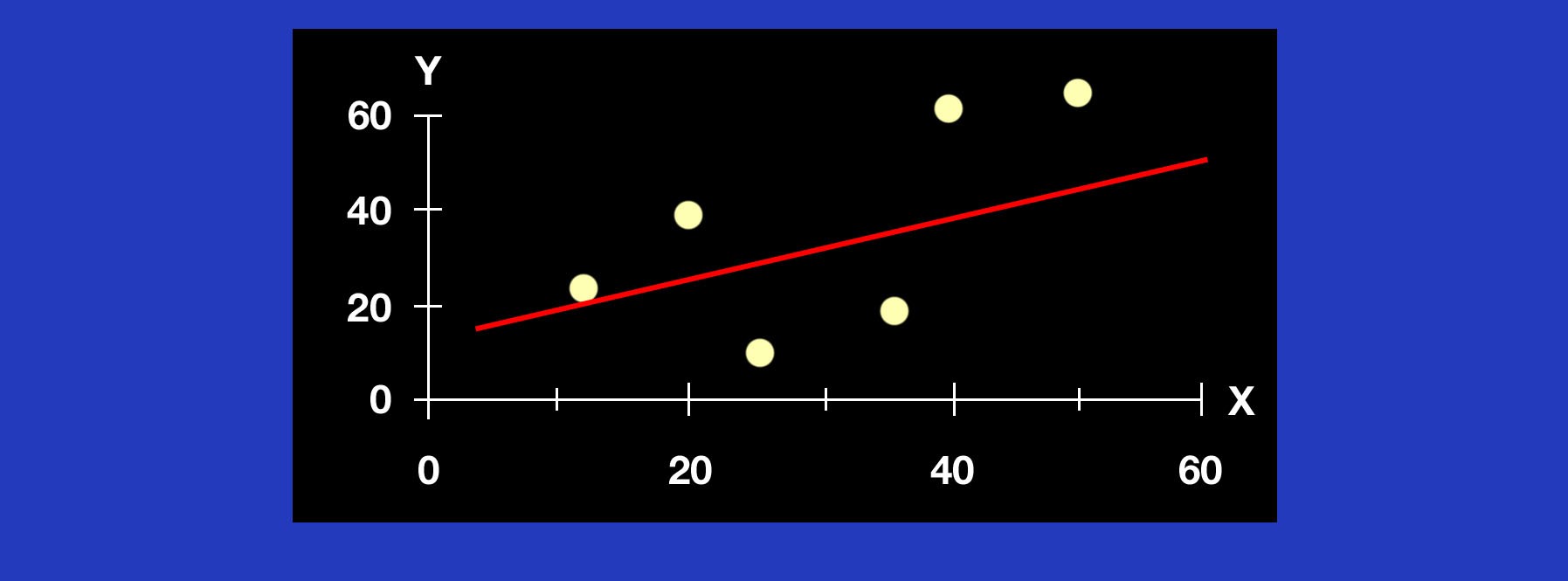
Figure 2.2 Line of best fit in regression analysis.
For a time series of n points of data where,
t = time i.e. the number of time periods from the starting point
y = the observed value in a given time period
The slope b of the line is given by:
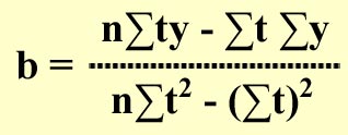 , and
, and
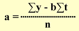
The intercept a is given by:
Interpretation of coefficients
Slope b is that the estimated Y changes by b, for each one unit increase in t.
Y-intercept (a) is the average value of Y when t = 0.
We will now look at a simple example for developing a linear trend equation using linear regression analysis for forecasting the trend component of a time series.